ACCEL² simulation

The Lyman-α forest and small-scale applications

Corentin Ravoux

Group presentation - 06/07/26


The Lyman-α forest


Corentin Ravoux                                                                                                                                                              Group presentation - July 6 2026

Quasars as back light sources

  • Quasar = supermassive black hole + accretion disk
  • Brightest objects in the Universe (up to 1000 x Milky Way)
  • High gravitational energy produced by the SMBH
  • Accretion disk, heating of matter by collisions
  • Observed up to z~7

Corentin Ravoux                                                                                                                                                              Group presentation - July 6 2026

The Lyman-α forest

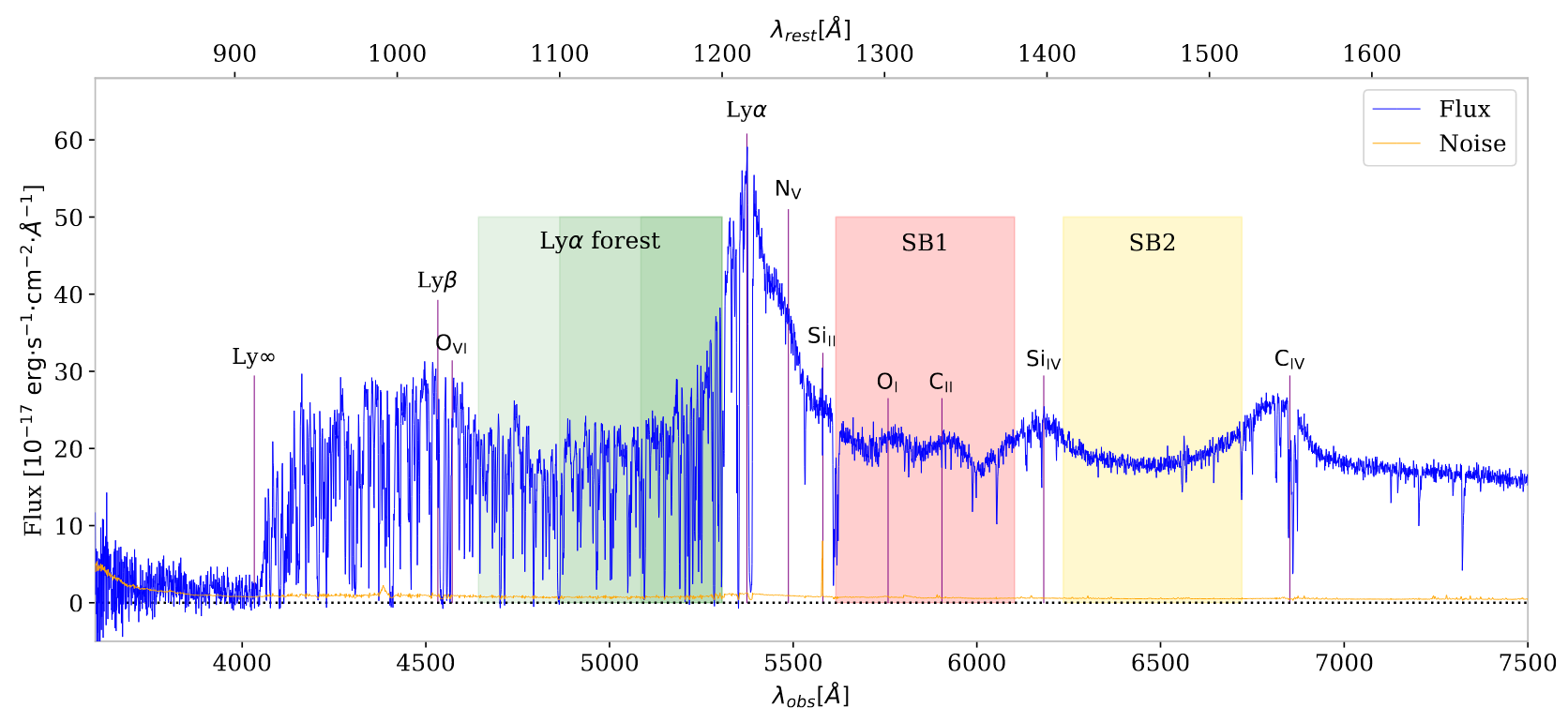
Wavelength [Angstrom]

Flux

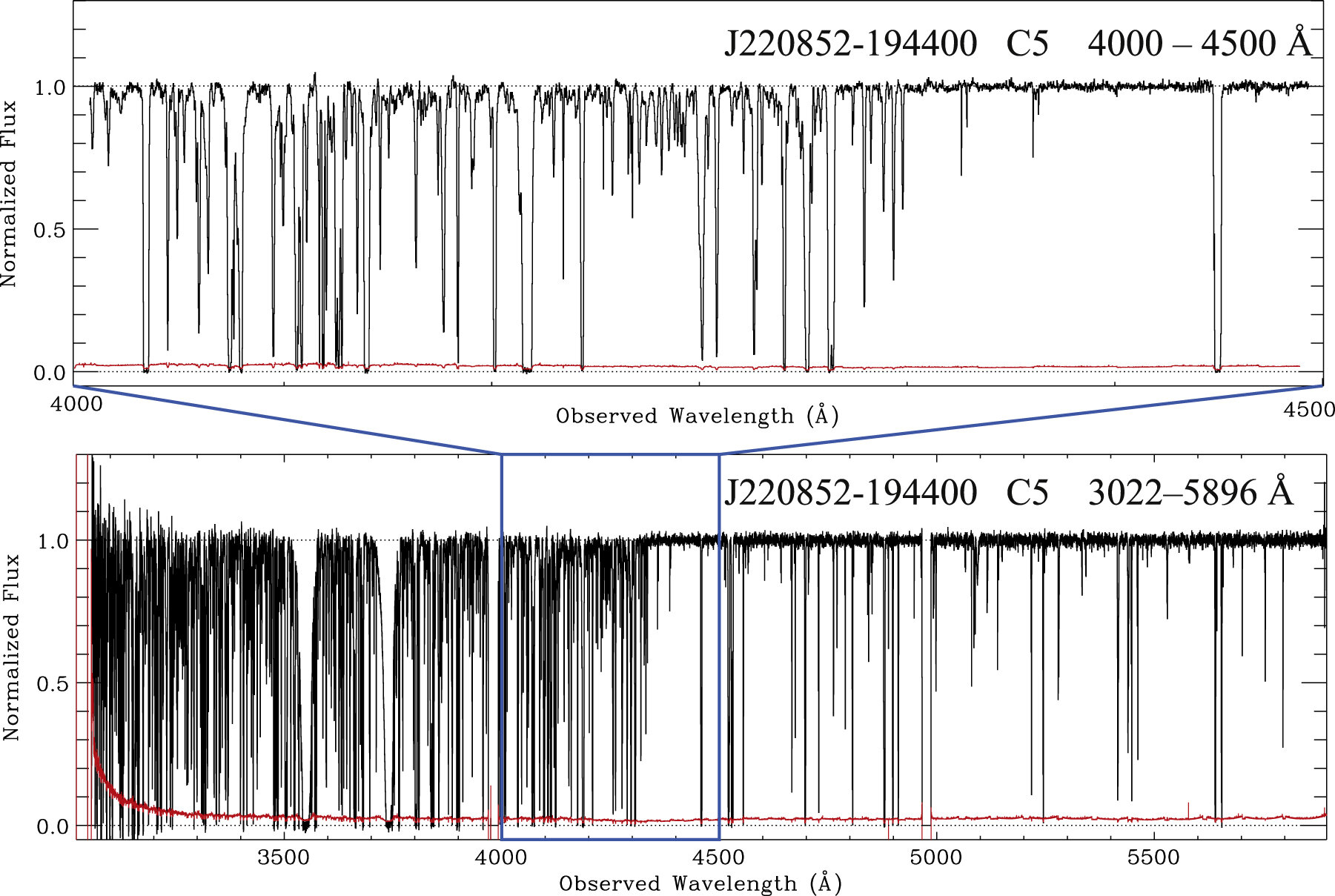
  • Lyman-α: transition of neutral Hydrogen to first excited state

  • Lines in quasar spectra at                                     caused by absorbers in the intergalactic medium (IGM) at
\lambda_{\mathrm{obs}} = (1 + z_{\mathrm{abs}}) \lambda_{\alpha}
z_{\mathrm{abs}}

DESI quasar at z =3.42

\lambda_{\alpha} = 121.567\ \mathrm{nm}

Ravoux et al. 2023

Corentin Ravoux                                                                                                                                                              Group presentation - July 6 2026
Corentin Ravoux                                                                                                                                                              Group presentation - July 6 2026

Lyman-α physics

\tau_\alpha(z)=\int n_{\mathrm{HI}}(z) \sigma_\alpha(z) d z
  • Lyman-α absorption optical depth:

Density of neutral hydrogen

Cross section of Lyman-α transition

  • Fraction of transmitted flux:
\mathrm{F}(z)= \frac{f_{\mathrm{out}}(z)}{C(z)}=\exp \left(-\tau_\alpha(z)\right)

F

Quasar continuum

Lyman-α forest = non-linear tracer of neutral hydrogen in the IGM at high redshifts (z>2)

Corentin Ravoux                                                                                                                                                              Group presentation - July 6 2026

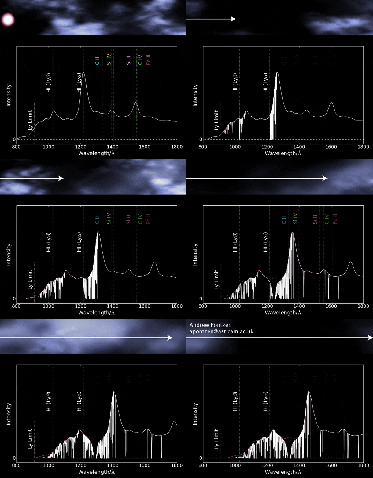
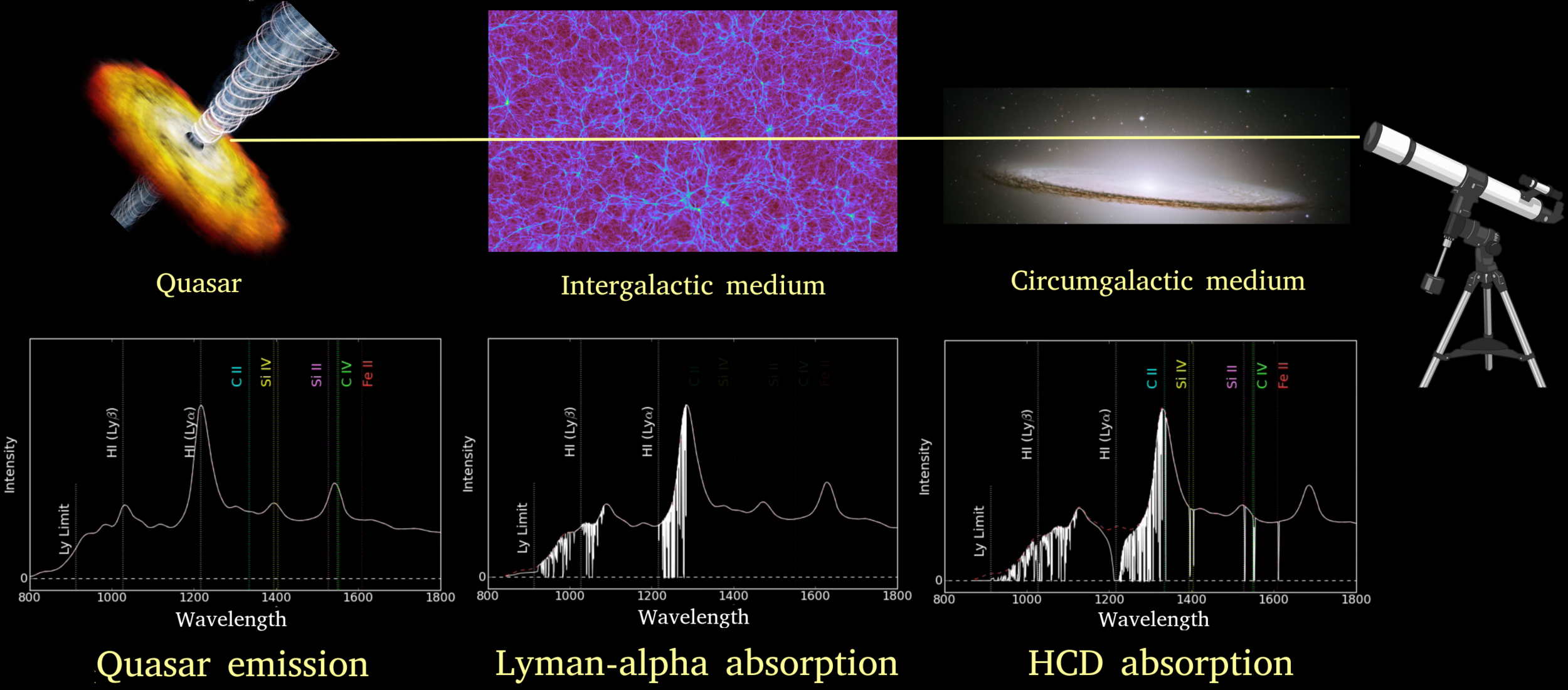
  • Near the quasar:
    • Unknown continuum
    • Broad absorption line quasars (BAL)

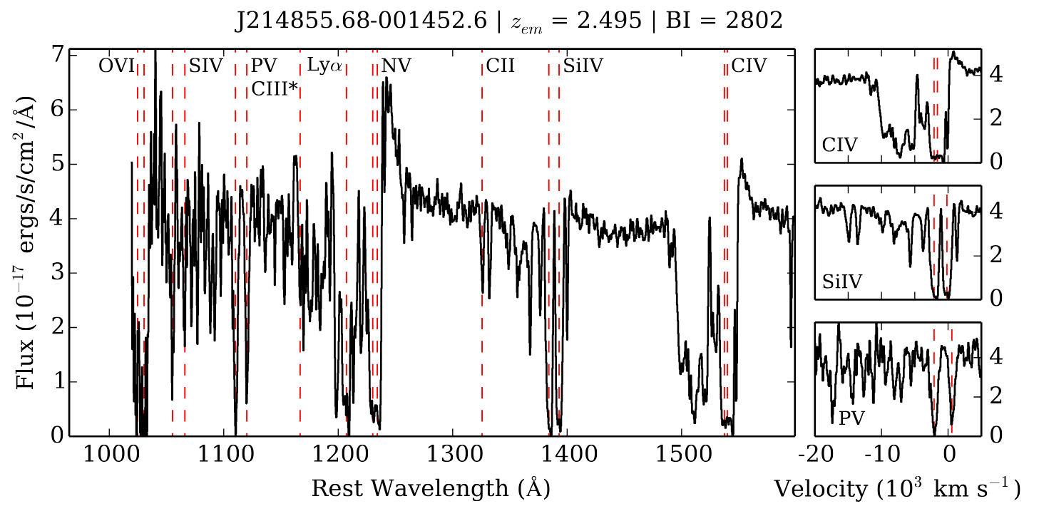
Contaminants

  • Along the line-of-sight:
    • Metal absorptions in the IGM
    • Damped Lyman-α systems (DLA)
  • Near the telescope:
    • Atmospheric absorption and emission
    • Instrument noise
    • Spectrograph resolution

Adapted from A. Pontzen video
Corentin Ravoux                                                                                                                                                              Group presentation - July 6 2026

Clustering with the Lyman-α forest


Corentin Ravoux                                                                                                                                                              Group presentation - July 6 2026

Quasar continuum
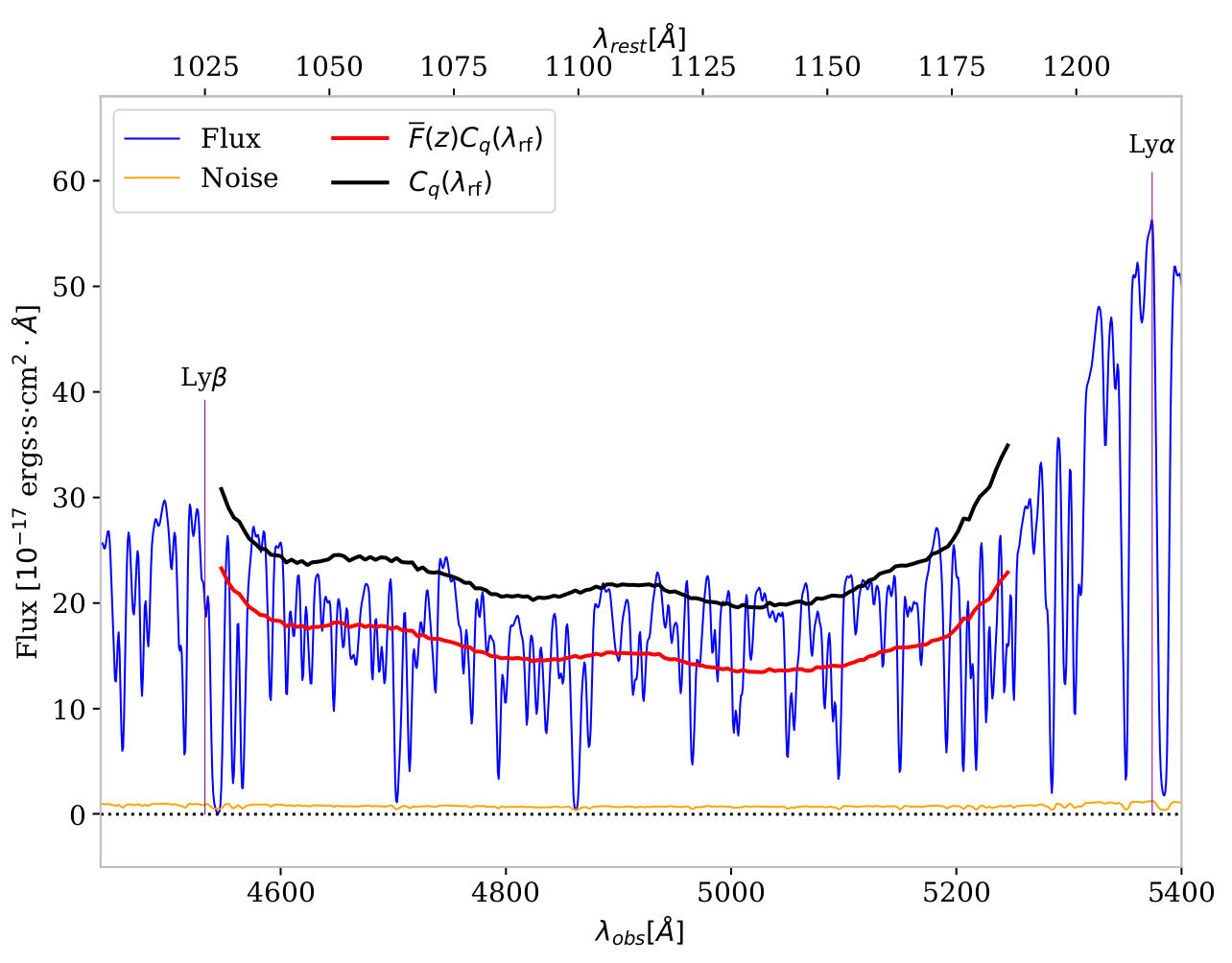
  • Quasar continuum: unknown and different for each quasar
  • Flux contrast (normalization):


Wavelength [Angstrom]

Flux

\begin{aligned} \delta_F(\lambda) &= \frac{F}{\overline{F}} - 1 \\ &= \frac{f(\lambda)}{\bar{F}(\lambda) C_{\mathrm{q}}\left(\lambda, z_{\mathrm{q}}\right)}-1 \end{aligned}

Corentin Ravoux                                                                                                                                                              Group presentation - July 6 2026

Definition of observational statistics

Configuration space

Fourier space

  • 3D auto-correlation:
\begin{aligned} &P_\alpha(\vec{k}) \delta_{\mathrm{D}}^{(3)}\left(\vec{k}+\vec{k^{\prime}}\right) \\ & =\frac{1}{(2 \pi)^3}\left\langle\delta_F(\vec{k}) \delta_F\left(\vec{k^{\prime}}\right)\right\rangle \end{aligned}
  • 3D power spectrum:
  • 1D power spectrum:
P_{1 \mathrm{D}, \alpha}\left(k_{\|}\right)=\int \frac{d \vec{k_{\perp}}}{(2 \pi)^2} P_\alpha\left(\vec{k}_{\perp}, k_{\|}\right)
\xi_{\alpha}(\vec{r})=<\delta_F(\vec{x}) \delta_F(\vec{x}+\vec{r})>_x
\xi_{\alpha X}(\vec{r})=<\delta_F(\vec{x}) \delta_X(\vec{x}+\vec{r})>_x
  • 3D cross-correlation:
  • 1D auto-correlation (not very used)
\vec{r}
\vec{k}
\xi_{1\mathrm{D},\alpha}(r_{\|})= <\delta_F(x) \delta_X(x+r_{\|})>_x

X = quasar, void

Corentin Ravoux                                                                                                                                                              Group presentation - July 6 2026

Lyman-α clustering

Observer

Quasar

Lyman-α forest

\vec{r_{\parallel}}
\vec{r_{\bot}}
\vec{r}
\theta
\mu = \cos \theta

Corentin Ravoux                                                                                                                                                              Group presentation - July 6 2026

Lyman-α clustering

Correlation

1D power spectrum (P1D)

Quasar

Lyman-α forest

1D auto correlation

Fourier space

Configuration space

P_{1 \mathrm{D}, \alpha}\left(k_{\|}\right)=\int \frac{d \vec{k_{\perp}}}{(2 \pi)^2} P_\alpha\left(\vec{k}_{\perp}, k_{\|}\right)
\xi_{1\mathrm{D},\alpha}(r_{\|})= <\delta_F(x) \delta_F(x+r_{\|})>_x
\vec{r_{\parallel}}
\vec{r_{\bot}}
\vec{r}
\theta
\mu = \cos \theta

Correlation

Corentin Ravoux                                                                                                                                                              Group presentation - July 6 2026

Lyman-α clustering

Correlation

Quasar

Lyman-α forest

\xi_{\alpha}(\vec{r})=<\delta_F(\vec{x}) \delta_F(\vec{x}+\vec{r})>_x
P_\alpha(\vec{k}) \delta_{\mathrm{D}}^{(3)}\left(\vec{k}+\vec{k^{\prime}}\right) =\frac{1}{(2 \pi)^3}\left\langle\delta_F(\vec{k}) \delta_F\left(\vec{k^{\prime}}\right)\right\rangle

3D power spectrum (P3D)

3D auto correlation

\vec{r_{\parallel}}
\vec{r_{\bot}}
\vec{r}
\theta
\mu = \cos \theta

Fourier space

Configuration space

Correlation

Corentin Ravoux                                                                                                                                                              Group presentation - July 6 2026

Lyman-α clustering

Configuration space

3D cross correlation with quasars

Correlation

Quasar

Lyman-α forest

\vec{r_{\parallel}}
\vec{r_{\bot}}
\vec{r}
\theta
\mu = \cos \theta
\xi_{\alpha q}(\vec{r})=<\delta_F(\vec{x}) \delta_q(\vec{x}+\vec{r})>_x

Corentin Ravoux                                                                                                                                                              Group presentation - July 6 2026

One-dimensional power spectrum (P1D)


Corentin Ravoux                                                                                                                                                              Group presentation - July 6 2026

Small scales

Large scales

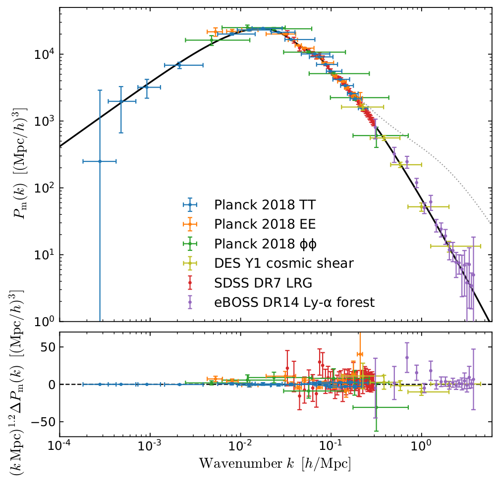
1D power spectrum (P1D)

  • Correlations along individual lines-of-sight

  • Sensitive to small-scale matter clustering and IGM thermal state

  • Probe the small-scale matter power spectrum


\Omega_{\mathrm{m}}, \sigma_8, n_s
A_{\mathrm{Ly\alpha}}, n_{\mathrm{Ly\alpha}}

Amplitude and slope at

z=3\ \&\ k=1\ h/ \mathrm{Mpc}

Chabanier et al. 2019

P1D range

Wavenumber k [Mpc^-1]

Matter power spectrum

One-dimensional power spectrum

Corentin Ravoux                                                                                                                                                              Group presentation - July 6 2026

Neutrino masses

\sum m_{\nu}

P1D range

CMB range

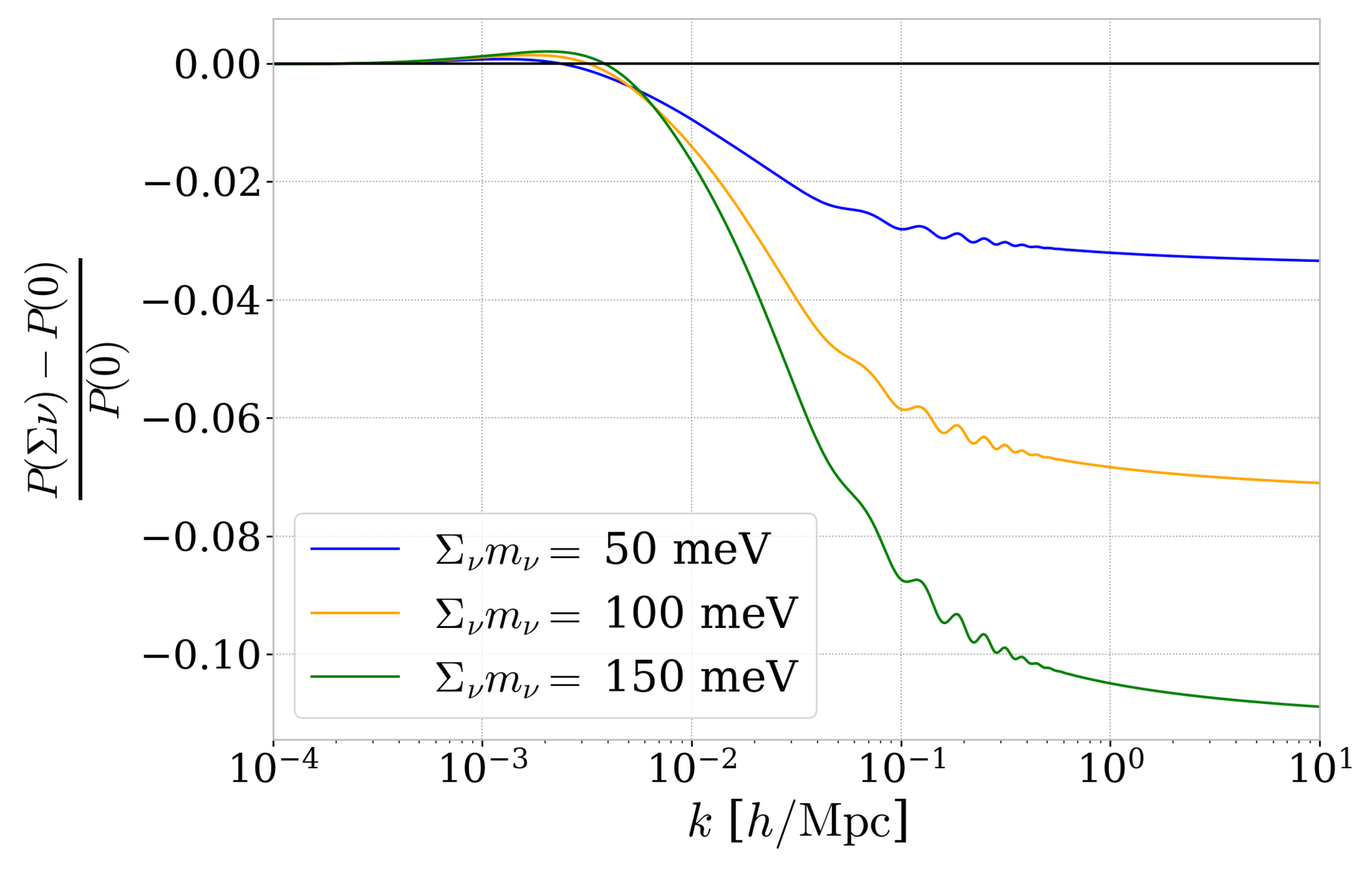
  • Oscillations experiments measure mass differences


  • Cosmology:
    • Neutrinos impact structure formation by smoothing matter power spectrum at small scales
    • Effect depends on the sum of neutrino masses

P1D constrain neutrino masses

Corentin Ravoux                                                                                                                                                              Group presentation - July 6 2026

  • Warm dark matter:
    • Thermal relics from cosmic microwave background
    • Mass-dependent power spectrum cut-off on small scales
  • Other models:
    • Fuzzy dark matter
    • Self-interacting dark matter
    • Primordial black holes

Dark matter properties

P1D range

Baur et al. 2015
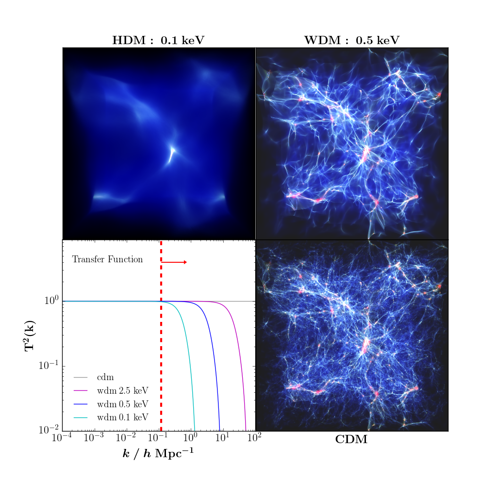
P1D constrain dark matter models

Corentin Ravoux                                                                                                                                                              Group presentation - July 6 2026

P1D estimator

  • P1D measured using Fast Fourrier Transform estimator
\begin{aligned} P_{1\mathrm{D},\alpha}(k) = & \left(\left\langle\left[P_{\mathrm{raw}}(k)-P_{\mathrm {pipeline}}(k) - \alpha \right] \cdot \mathbf{R}^{-2}(k) \right\rangle - P_{\mathrm{SB1,m}}(k) \right) \\ & \cdot A_{\mathrm{line}}(z,k) \cdot A_{\mathrm{dla}}(z,k) \cdot A_{\mathrm{cont}}(z,k) \cdot A_{\mathrm{res}}(k) \end{aligned}
= \left\langle|\delta_F(k)|^2\right\rangle
\big \rangle
\delta_F(k)

Without correction, Fourier transform of flux contrasts and averaging for all quasars

Corentin Ravoux                                                                                                                                                              Group presentation - July 6 2026

P1D estimator

  • P1D measured using Fast Fourrier Transform estimator
\begin{aligned} P_{1\mathrm{D},\alpha}(k) = & \left(\left\langle\left[P_{\mathrm{raw}}(k)-P_{\mathrm {pipeline}}(k) - \alpha \right] \cdot \mathbf{R}^{-2}(k) \right\rangle - P_{\mathrm{SB1,m}}(k) \right) \\ & \cdot A_{\mathrm{line}}(z,k) \cdot A_{\mathrm{dla}}(z,k) \cdot A_{\mathrm{cont}}(z,k) \cdot A_{\mathrm{res}}(k) \end{aligned}

Correction of the noise estimation

Spectroscopic resolution correction

Corentin Ravoux                                                                                                                                                              Group presentation - July 6 2026

P1D estimator

  • P1D measured using Fast Fourrier Transform estimator
\begin{aligned} P_{1\mathrm{D},\alpha}(k) = & \left(\left\langle\left[P_{\mathrm{raw}}(k)-P_{\mathrm {pipeline}}(k) - \alpha \right] \cdot \mathbf{R}^{-2}(k) \right\rangle - P_{\mathrm{SB1,m}}(k) \right) \\ & \cdot A_{\mathrm{line}}(z,k) \cdot A_{\mathrm{dla}}(z,k) \cdot A_{\mathrm{cont}}(z,k) \cdot A_{\mathrm{res}}(k) \end{aligned}

Measurement of  absorption from other IGM elements

Correction of the noise estimation

Spectroscopic resolution correction

Corentin Ravoux                                                                                                                                                              Group presentation - July 6 2026

P1D estimator

  • P1D measured using Fast Fourrier Transform estimator
\begin{aligned} P_{1\mathrm{D},\alpha}(k) = & \left(\left\langle\left[P_{\mathrm{raw}}(k)-P_{\mathrm {pipeline}}(k) - \alpha \right] \cdot \mathbf{R}^{-2}(k) \right\rangle - P_{\mathrm{SB1,m}}(k) \right) \\ & \cdot A_{\mathrm{line}}(z,k) \cdot A_{\mathrm{dla}}(z,k) \cdot A_{\mathrm{cont}}(z,k) \cdot A_{\mathrm{res}}(k) \end{aligned}

Masking of atmospheric lines

Masking of Damped Lyman-α systems

Correction of continuum fitting error

Correction of the noise estimation

Spectroscopic resolution correction

Measurement of  absorption from other IGM elements

Correction of the resolution estimation

All corrections derived from simulation or models

Corentin Ravoux                                                                                                                                                              Group presentation - July 6 2026

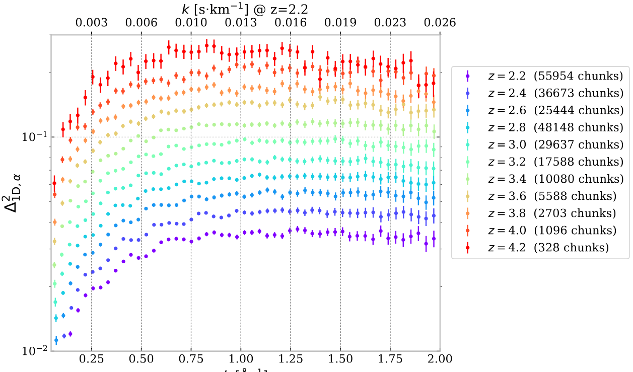
P1D measurements on DESI DR1

P1D

Wavenumber k [Ang^-1]

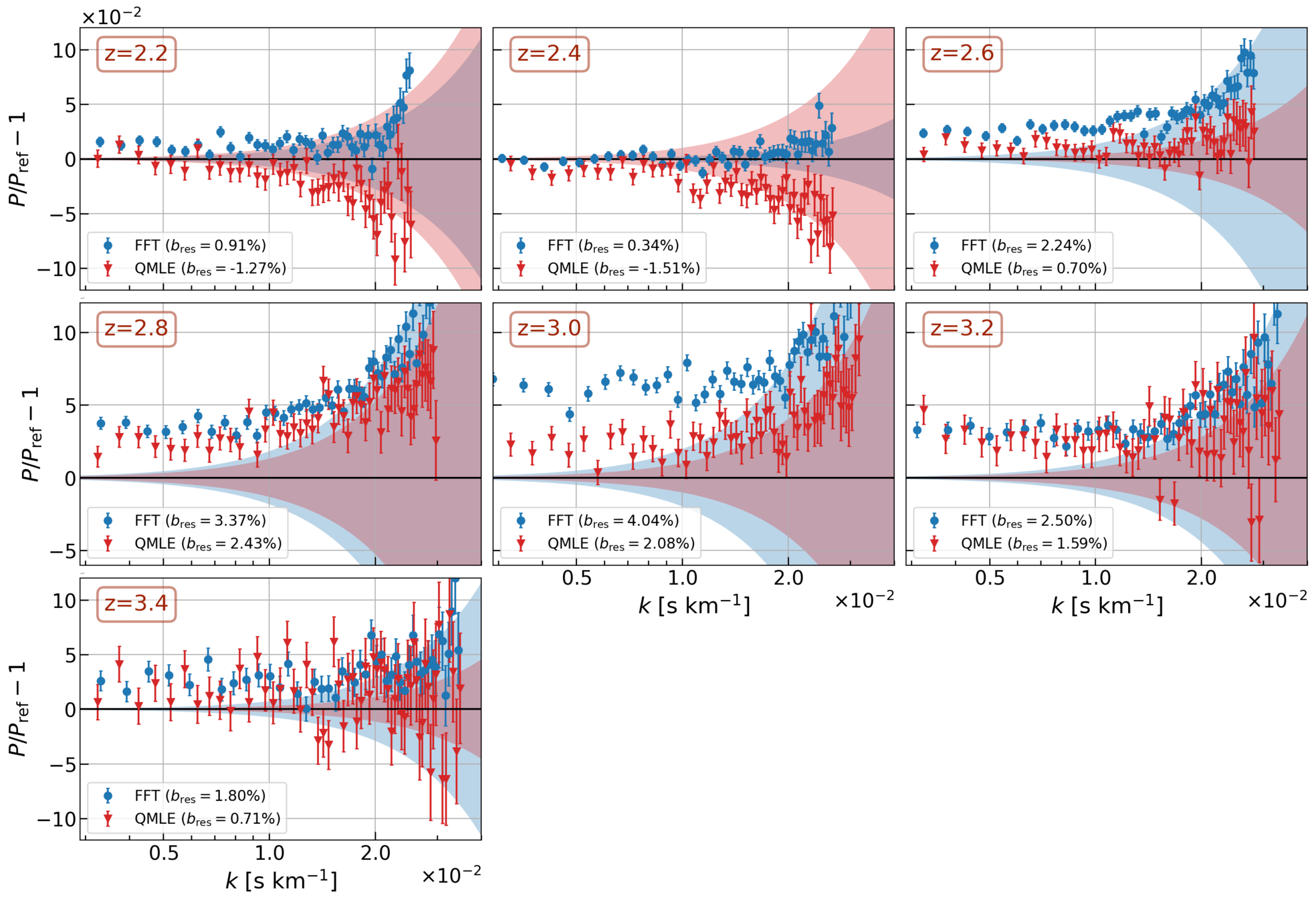
  • DESI DR1 measurement
  • Large number of quasars (159132) with rather noisy spectra = small statistical error
  • Error bars accounting for systematic and statistical uncertainties

Ravoux et al. 2025
Corentin Ravoux                                                                                                                                                              Group presentation - July 6 2026

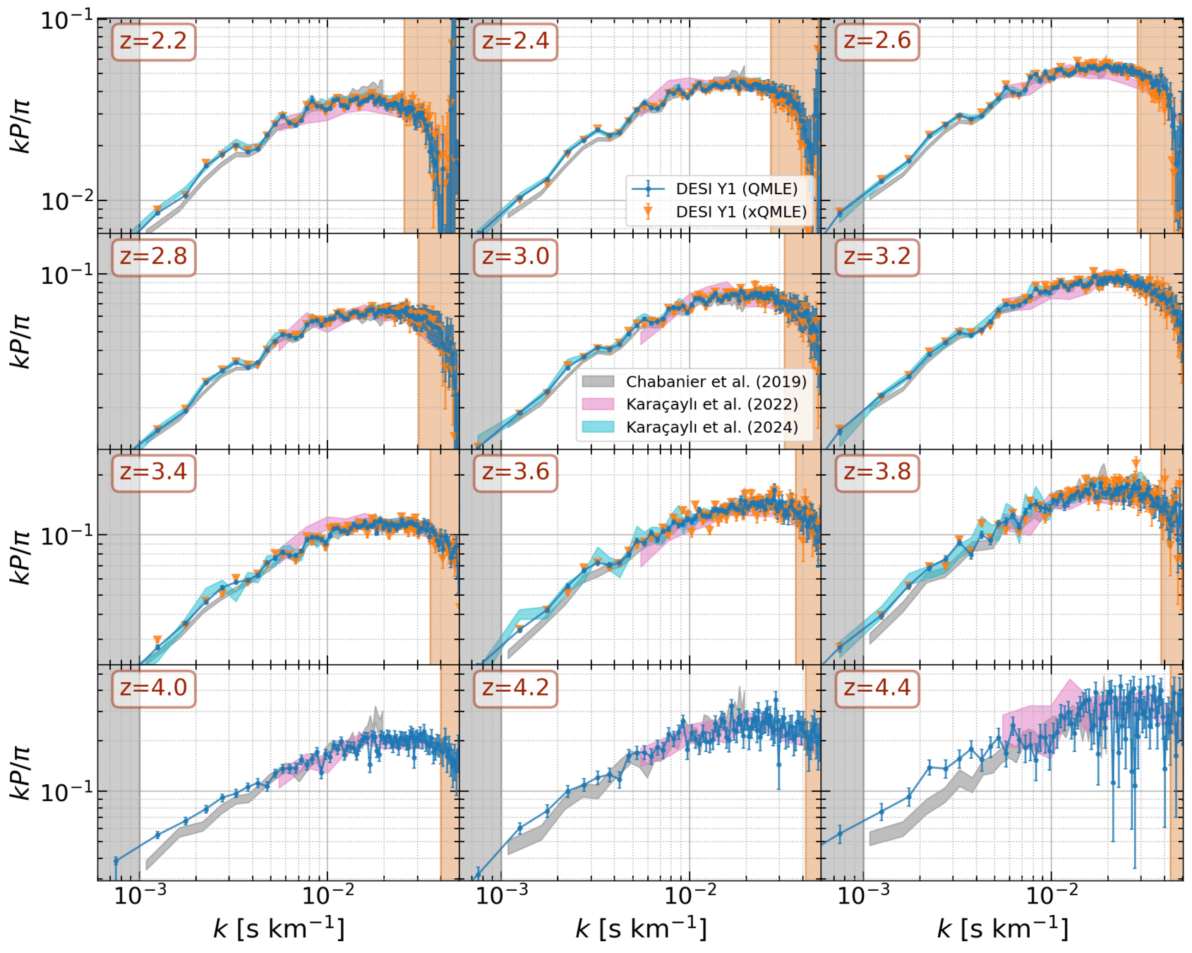
Alternative measurement: QMLE

  • QMLE = Quadratic Maximum Likelihood Estimator
  • Covariance from theory and P1D estimate, minimized through likelihood
  • Same dataset, different method and systematic treatment
\mathcal{L}\left(\delta_F; P_{1 \mathrm{D}, \alpha}\right)=-\ln (\operatorname{det}(\mathbf{C}))-\delta_F^\mathrm{T} \cdot \mathbf{C}^{-1} \cdot \delta_F

Karacaylı et al. 2025

Corentin Ravoux                                                                                                                                                              Group presentation - July 6 2026

Estimator comparison

  • Full comparison of FFT and QMLE methods on:
    • DESI-like mocks
    • Pixel-level simulations
  • Validation of both estimators regarding all contaminants
  • Full detail of the systematic budget
  • DR1 data agreement

Karacaylı, Ravoux et al. 2025

Corentin Ravoux                                                                                                                                                              Group presentation - July 6 2026

Modeling: High-resolution simulations
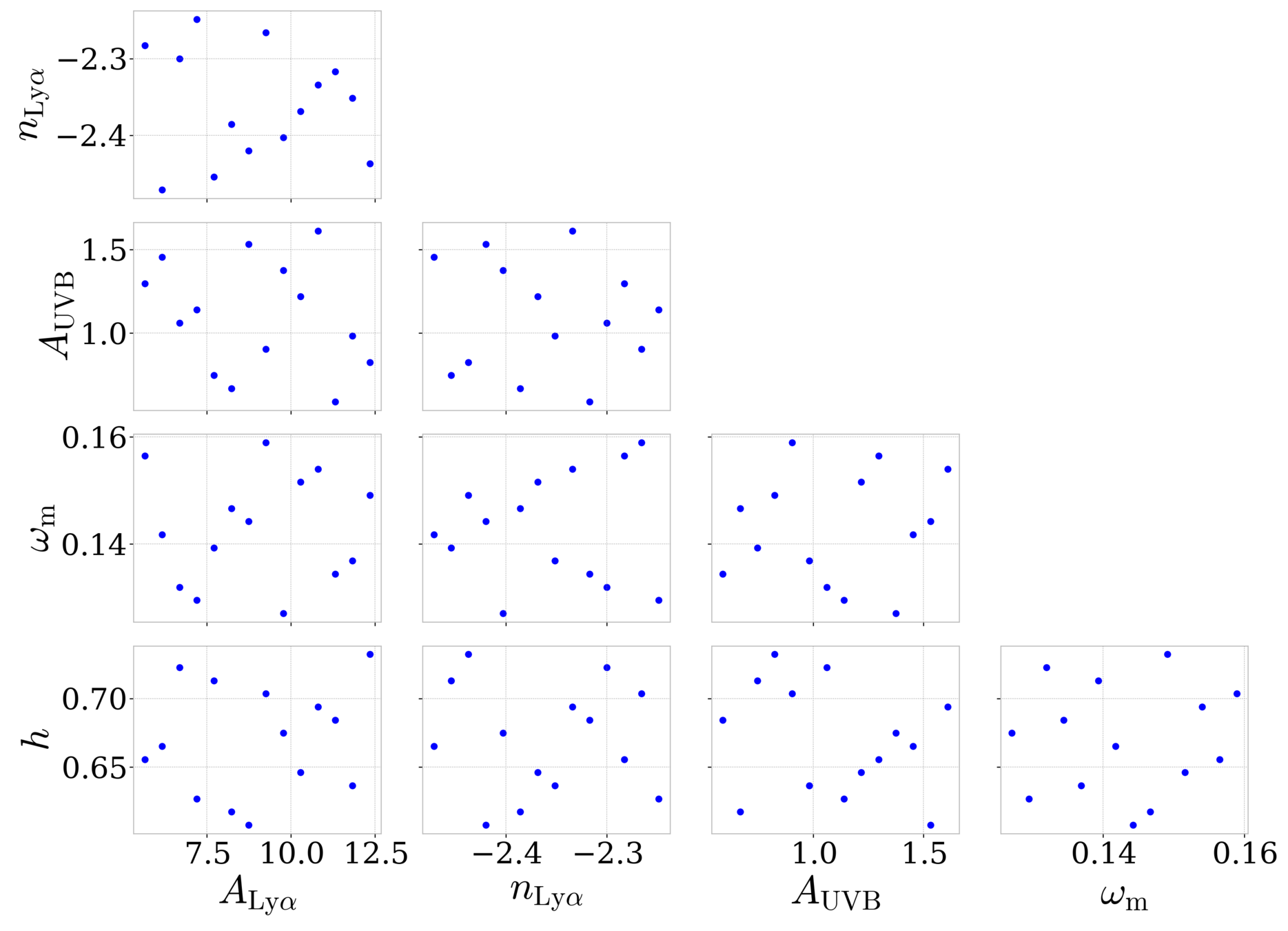
  • Interpretation of P1D measurement with high-resolution hydrodynamical simulations (very expensive)


  • Issue: each simulation takes ~10⁵ CPU hours or ~ 1000 GPU hours

Walther et al. 2021

Corentin Ravoux                                                                                                                                                              Group presentation - July 6 2026

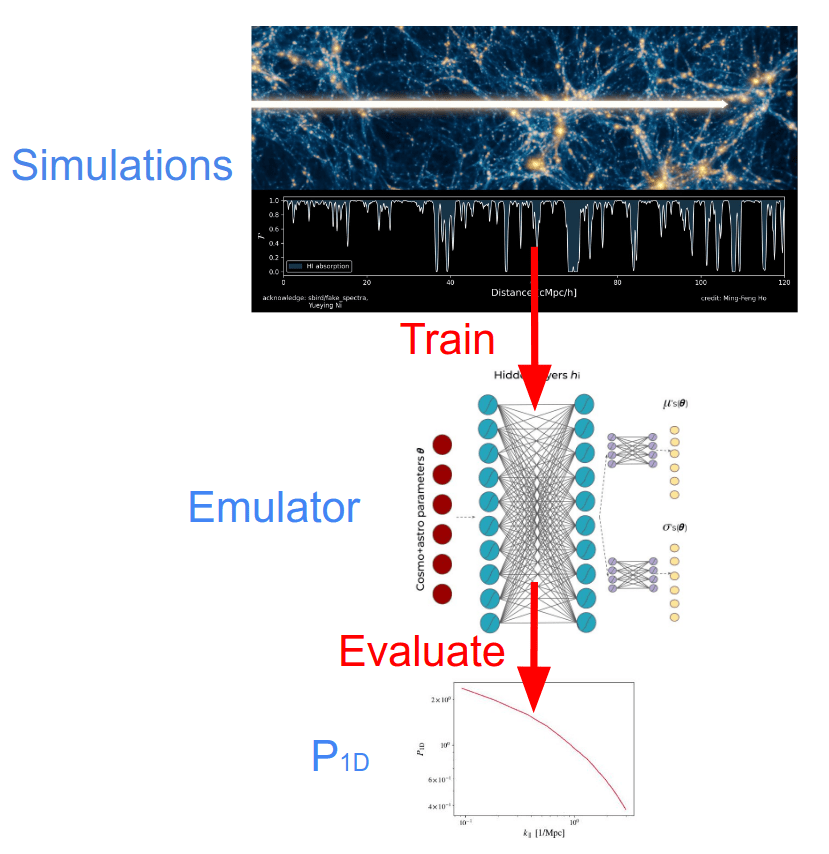
Modeling: DESI emulators

  • Two simulation grids built:
    • Nyx (full hydro)
    • MP-Gadget (SPH particles)
  • Gaussian processes
    emulators with adapted
    cosmological/IGM parameters
    • Interpolation between simulations
    • Covers cosmological parameter space evenly
    • Include IGM thermal state marginalization
Cabayol-Garcia  et al. 2023

Walther et al. 2021

Walther et al. 2025

Pedersen et al. 2023

Pedersen et al. 2021

Corentin Ravoux                                                                                                                                                              Group presentation - July 6 2026

DESI DR1 constraints: fit
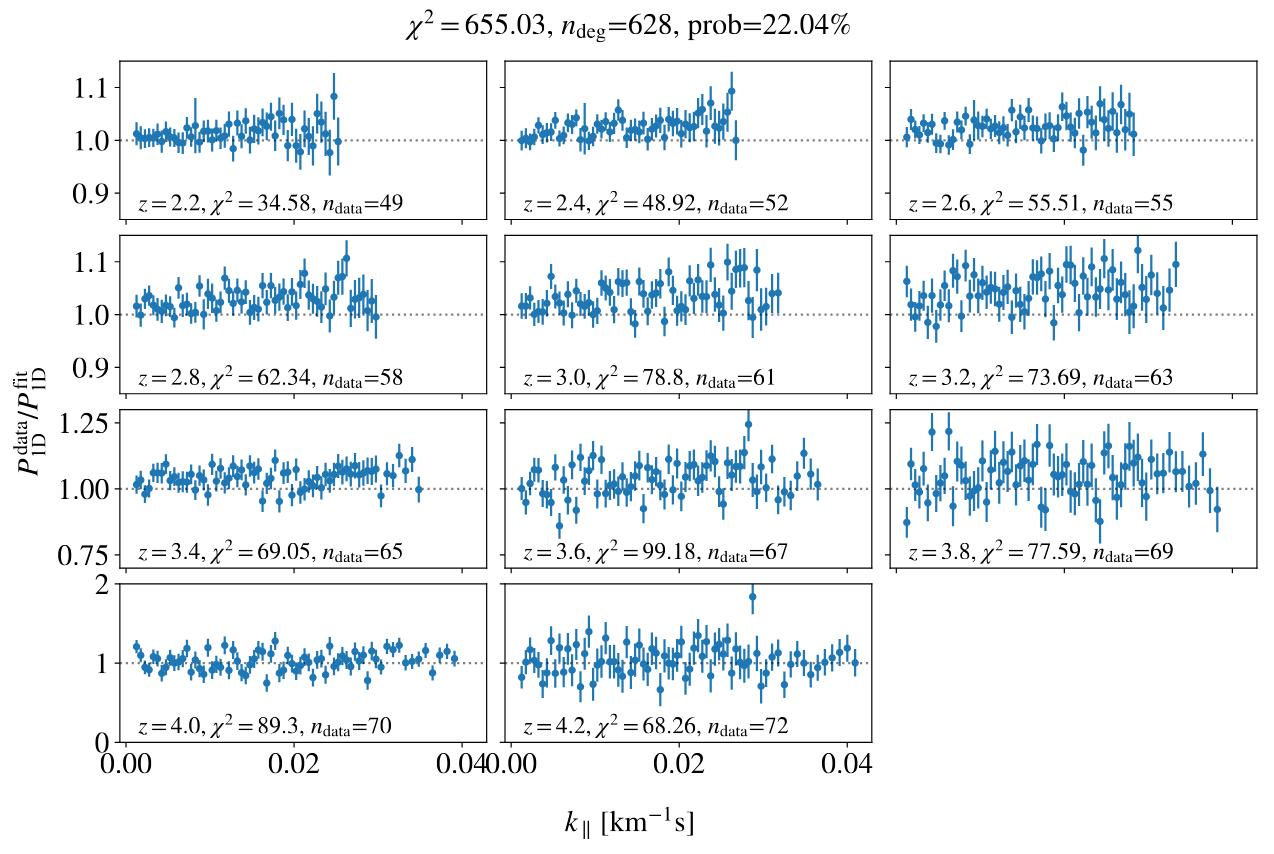
  • Extensive effort on main contaminant modeling:
    • metal correlations
    • DLA contamination
    • spectrograph resolution
    • IGM thermal state
  • Combination of both DR1 measurements 

Chaves-Montero et al. 2025

Corentin Ravoux                                                                                                                                                              Group presentation - July 6 2026

DESI DR1 constraints: Primordial power spectrum
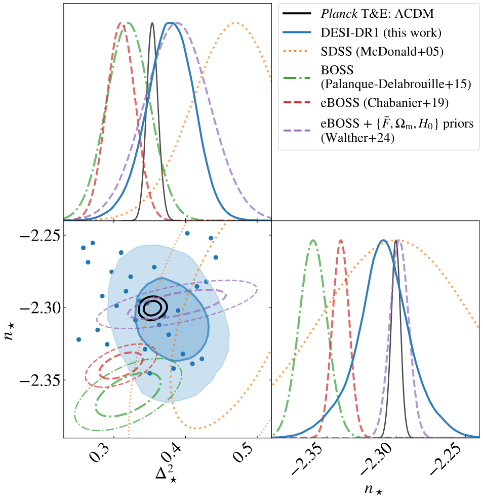
\begin{aligned} & \log \Delta_{\mathcal{R}}^2(k)=\log A_{\mathrm{s}}+\left(n_{\mathrm{s}}-1\right) \log \left(k / k_{\mathrm{s}}\right) \\ \end{aligned}
  • Expressing primordial power spectrum amplitude (     or     ) and index (    ) at the scale and redshift of P1D: bijective transformation
  • Large error bar from conservative systematics and emulator errors 
  • In agreement with eBOSS
A_\mathrm{s}
n_\mathrm{s}
\sigma_8

Chaves-Montero et al. 2025

Corentin Ravoux                                                                                                                                                              Group presentation - July 6 2026

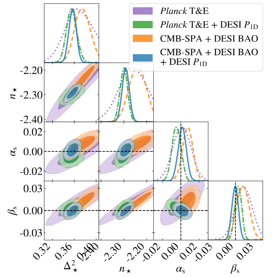
DESI DR1 constraints: Inflation

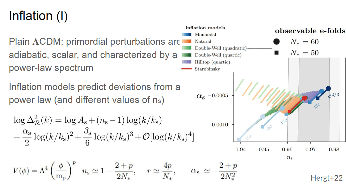
\begin{aligned} & \log \Delta_{\mathcal{R}}^2(k)=\log A_{\mathrm{s}}+\left(n_{\mathrm{s}}-1\right) \log \left(k / k_{\mathrm{s}}\right) \\ & +\frac{\alpha_{\mathrm{s}}}{2} \log \left(k / k_{\mathrm{s}}\right)^2+\frac{\beta_{\mathrm{s}}}{6} \log \left(k / k_{\mathrm{s}}\right)^3 \end{aligned}
  • Relaxing slope variation for primordial power spectrum = constraints on inflation models
  • Improve Planck constraints

Chaves-Montero et al. 2025

Corentin Ravoux                                                                                                                                                              Group presentation - July 6 2026

DESI DR1 constraints: Neutrinos
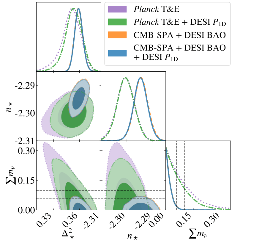
  • Large constraints by comparing probes of large scales (CMB) with small scale ones (P1D)
  • Does not improve much the DESI DR2 BAO constraints but:
    • P1D constraints from LSS not evolution (BAO)

Chaves-Montero et al. 2025

Corentin Ravoux                                                                                                                                                              Group presentation - July 6 2026

DESI DR1 constraints: summary
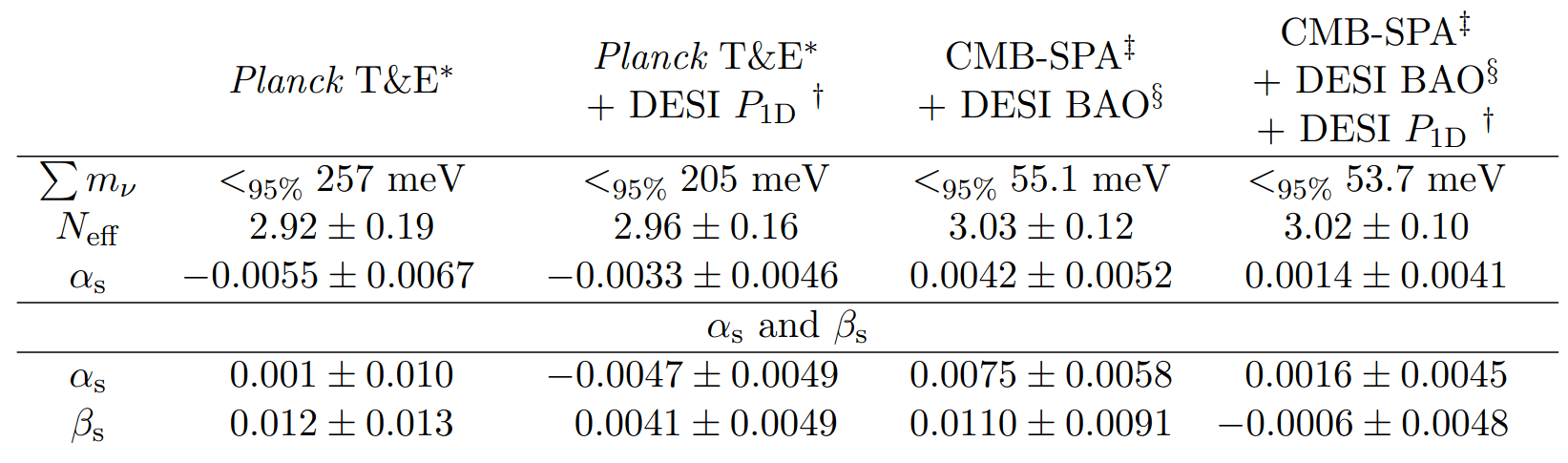
Chaves-Montero et al. 2026

  • P1D DR1 is systematics dominated: efforts for reducing measurements and emulators systematics for next measurements (DR3)

Corentin Ravoux                                                                                                                                                              Group presentation - July 6 2026

DESI DR3 forecasts

\sigma\left(\sum m_{\nu}\right) = 0.03~\mathrm{eV}
  • Constraints on WDM improved by a factor 1.6
  • IGM thermal parameters by a factor 2.
  • Neutrino mass, in association with BAO and CMB:

 Valluri et al. 2022
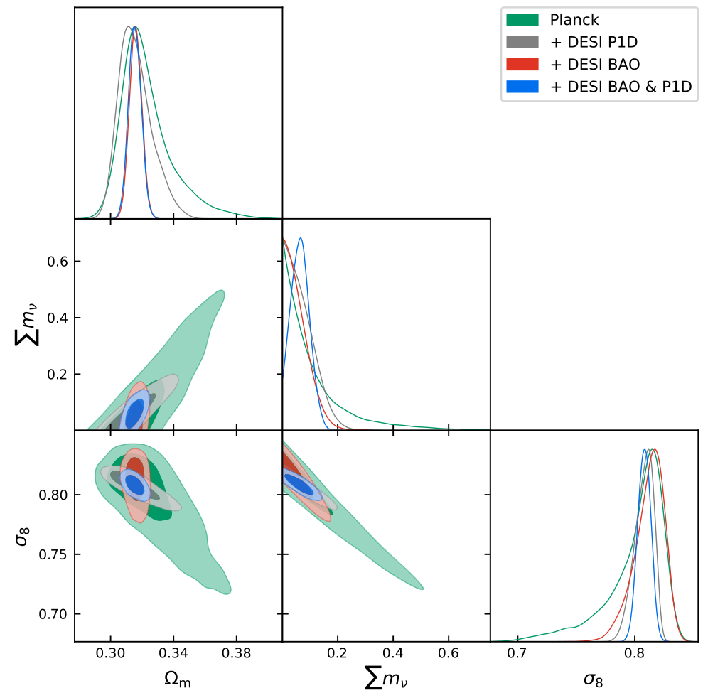
Credits to A. Font-Ribera

Preliminary

Corentin Ravoux                                                                                                                                                              Group presentation - July 6 2026

Future of Fourier space measurements

3D power spectrum

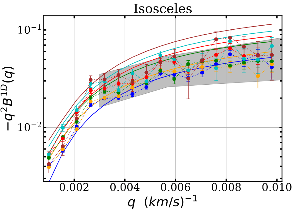
Bispectrum

  • 3-point correlation function in Fourier space = more information from cosmic web
  • 3D information in Fourier space
  • Made complicated by the intrinsic anisotropy of the Lyman-α forest
  • 3-point correlation function in Fourier space = more information from cosmic web

 de la Cruz et al. 2024
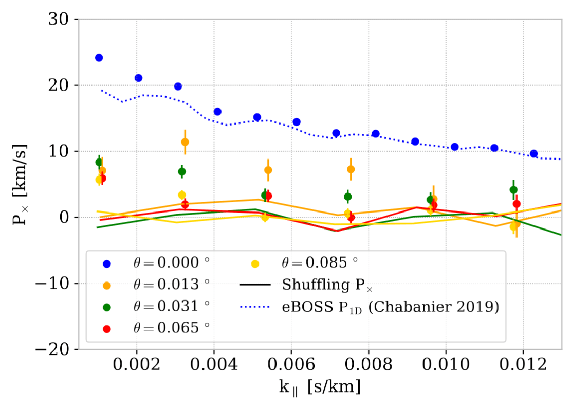
Abdul Karim et al. 2023

+ Work on P1D interpretation with EFTofLSS theories (Karacaylı et al. 2026)

Corentin Ravoux                                                                                                                                                              Group presentation - July 6 2026

Conclusion

  • Lyman-α forest = probe of IGM small scales and thermal state
  • P1D DESI DR1 measurement: encouraging constraints, need to be improved in the next measurements
  • A lot of related applications (P3D, B1D, EFT constraints...)

ACCEL² simulation
Gunn-Peterson effect

  • Universe is expanding: Hubble velocity flow
  • The matter has peculiar velocity
\mathrm{v}=\mathrm{c}\left[\nu_\alpha / \nu-1\right] = c z
\tau_\alpha(\mathrm{v})=\left(\frac{\sqrt{\pi} e^2}{m_{\mathrm{e}}}\right)\left(\frac{1}{4 \pi \epsilon_0}\right) \lambda_\alpha f_\alpha \int n_{\mathrm{HI}}\left(\mathrm{v}^{\prime}\right) \frac{1}{b\left(\mathrm{v}^{\prime}\right) H\left(\mathrm{v}^{\prime}\right)} e^{-\left(\frac{\mathrm{v}-\mathrm{v}^{\prime}-\mathrm{v}_{\|}\left(\mathrm{v}^{\prime}\right)}{b\left(\mathrm{v}^{\prime}\right)}\right)^2} d \mathrm{v}^{\prime}
\mathrm{v}_{\|}

Velocity space:

  • Complete calculation gives:

Density of neutral hydrogen/baryon

Doppler parameter (depends on temperature)

Universe expansion

IGM peculiar velocity

Fluctuating Gunn-Peterson approximation

  • IGM thermal equilibrium + highly photoionized + optically thin approximation + larges scales (> 2 Mpc):
\tau_\alpha(z) \propto \frac{(1+z)^6}{H(z)} \times (1+\eta(z))^{-1} \times T(z)^{-0.7} \times \Omega_{\mathrm{b}}^2\left(1+\delta_{\mathrm{b}}(z)\right)^\beta

Density of neutral hydrogen/baryon

Peculiar velocities

Universe expansion

Universe temperature

Lyman-α forest = non-linear tracer of neutral hydrogen in the IGM

  • At high redshift (z >2), fraction of neutral hydrogen

Lyman-α forest observable from the ground

x_{\mathrm{HI}} \sim 10^{-5} \longrightarrow \tau_{\alpha} \sim 1

Intermediate resolution: eBOSS (2014 - 2019)
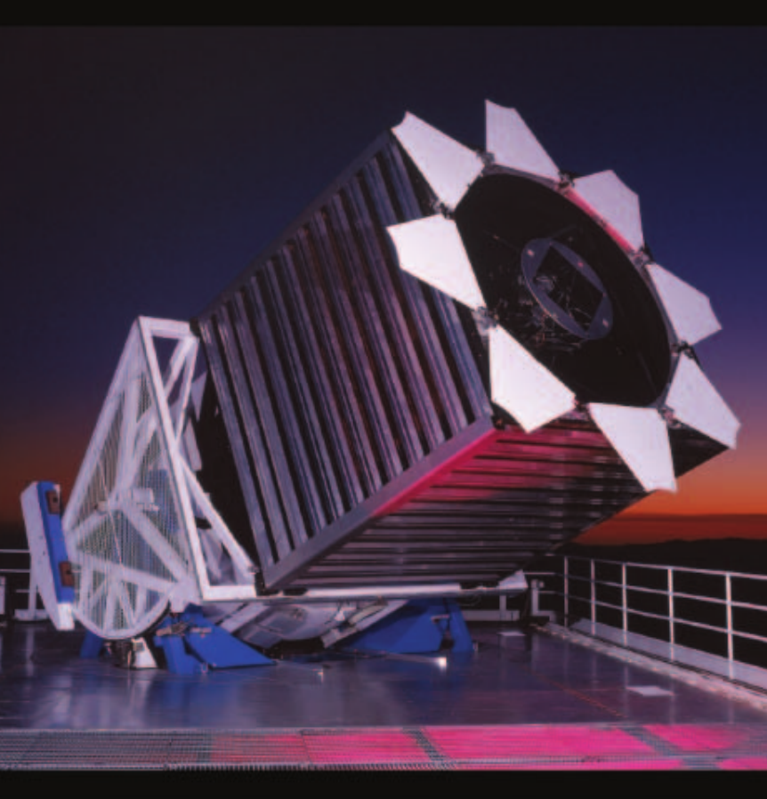
  • Multi-object spectrograph
  • 2.5 m telescope at Apache Point Observatory
  • 210 000 Lyman-α forests

Quasar continuum fit

  • Several methods:
    • Using very high resolution quasar spectra/stack of spectra
    • Principal Component Analysis template decomposition
    • Measuring on hydro simulation
    • Brute force: Likelihood minimization of a common model
C_{\mathrm{q}}\left(\lambda, z_{\mathrm{q}}\right)=\left(a_{\mathrm{q}}+b_{\mathrm{q}} \Lambda\right) C\left(\lambda_{\mathrm{rf}}=\frac{\lambda}{\left(1+z_{\mathrm{q}}\right)}\right)
\mathcal{L}=-\sum_i \frac{\left[f_i-\bar{F}\left(\lambda_i\right) C_{\mathrm{q}}\left(\lambda_i, z_{\mathrm{q}}, a_{\mathrm{q}}, b_{\mathrm{q}}\right)\right]^2}{\sigma_{\mathrm{q}}^2\left(\lambda_i\right)}-\ln \left[\sigma_{\mathrm{q}}^2\left(\lambda_i\right)\right]

picca python package

Common continuum model

Flux noise renormalized

\delta_F(\lambda)

Contaminants: Broad absorption line quasars

Adapted from A. Pontzen video

  • BAL quasars: Absorptions occuring inside the quasar (non-IGM = contaminant)
  • High velocity outflows from the quasar torus
  • Absorption from one or several clouds of gas
  • ~15 % of quasars

Capellupo et al. 2017

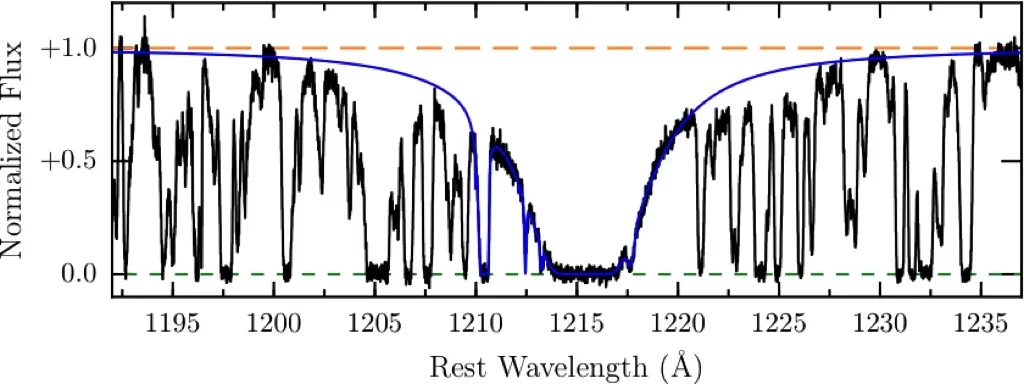
Contaminants: Damped Lyman-α systems

  • DLA: passing of the QSO light in the circum-galactic medium
  • Oversaturated absorption impacts a large spectra portion = clustering contaminant
  • Present on 30-40% of the quasars

Cooke et al. 2017

Contaminants: Metal absorptions

Adapted from A. Pontzen video

  • Metals: Other elements present in the IGM (Si, C, N, O...)
  • Like hydrogen, every element has a forest associated to each line
  • Depends a lot on the IGM proportion of each elements
F = \left(F_{\mathrm{Ly}\alpha} + F_{\mathrm{Si_{IV}}} + F_{\mathrm{C_{IV}}} + ..... \right.

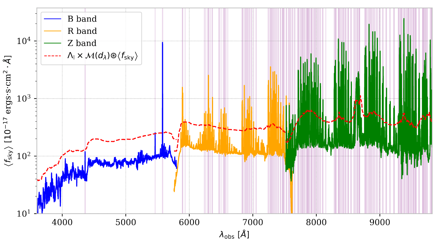
Contaminants: Instrument

Adapted from A. Pontzen video

  • Atmosphere:
    • Absorptions reduces the signal in the UV
    • Emission lines bias the clustering
  • Noise:
    • Very various sources (Poisson, electronic, calibration images...)
    • Hard to model
  • Spectral resolution:
    • Ability to distinguish two consecutive lines
    • Smooth the thinnest lines in the signal
F = \left(F_{\mathrm{Ly}\alpha} + F_{\mathrm{Si_{IV}}} + F_{\mathrm{C_{IV}}} + ..... + N \right) \circledast W\left(\lambda, R\right)
R = \lambda / \Delta \lambda

Resolution power

Ravoux et al. 2023

Correlation estimator

  • Need to discretize the statistic:
\vec{r_{\bot}}
\vec{r_{\parallel}}
\vec{r}
\vec{r}

Bin A

\xi_{\alpha}(\vec{r})=<\delta_F(\vec{x}) \delta_F(\vec{x}+\vec{r})>_x
  • Estimator for auto-correlation:
\hat{\xi}_{\alpha}(A)=\frac{\sum_{(i, j) \in A} w_i w_j \delta_{F}^i \delta_{F}^j}{\sum_{(i, j) \in A} w_i w_j}
  • Run over Lyman-alpha forest quasars, can be computationally expensive
  • Similar estimator with point-like contrast for quasar, voids, galaxies...

= pixel weights from continuum fitting

w_i
\delta_{F}^i
\delta_{F}^j

Modeling: theoretical model

P_{XY}(k, \mu)=b_X b_Y\left(1+\beta_X \mu^2\right)\left(1+\beta_Y \mu^2\right) P_{\mathrm{L}}(k,\mu)
  • Model for correlation between tracer X and Y:

Linear perturbation theory (Kaiser)

Tracer biases

RSD parameters

Linear power spectrum

Modeling: theoretical model

P_{XY}(k, \mu)=b_X b_Y\left(1+\beta_X \mu^2\right)\left(1+\beta_Y \mu^2\right) P_{\mathrm{QL}}(k,\mu)
  • Model for correlation between tracer X and Y:

Power spectrum modified

P_{\mathrm{QL}}(k,\mu, z)=P_{\mathrm{sm}}(k)+\exp \left[-\frac{k_{\|}^2 \Sigma_{\|}^2+k_{\perp}^2 \Sigma_{\perp}^2}{2}\right] P_{\text {peak }}(k)

Modeling: theoretical model

P_{XY}(k, \mu)=b_X b_Y\left(1+\beta_X \mu^2\right)\left(1+\beta_Y \mu^2\right) P_{\mathrm{QL}}(k,\mu)
  • Model for correlation between tracer X and Y:

Power spectrum modified

P_{\mathrm{QL}}(k,\mu, z)=P_{\mathrm{sm}}(k)+\exp \left[-\frac{k_{\|}^2 \Sigma_{\|}^2+k_{\perp}^2 \Sigma_{\perp}^2}{2}\right] P_{\text {peak }}(k)

Smooth component (no BAO)

BAO damping due to non-linear clustering

BAO component (wiggles)

k_{\|}=k_{\|}^{\mathrm{fid}} / \alpha_{\|}
k_{\bot}=k_{\bot}^{\mathrm{fid}} / \alpha_{\bot}
  • Parameters introduced by rescaling:

Modeling: theoretical model

P_{XY}(k, \mu)=b_X b_Y\left(1+\beta_X \mu^2\right)\left(1+\beta_Y \mu^2\right) P_{\mathrm{QL}}(k,\mu) F_{\mathrm{NL}}(k,\mu) G(k,\mu)
  • Model for correlation between tracer X and Y:

Correction for binning

Non-linear Lyman-α clustering correction

D_1(k, \mu)=\exp \left\{\left[q_1 \Delta^2(k)+q_2 \Delta^4(k)\right]\left[1-\left(\frac{k}{k_v}\right)^{a_v} \mu^{b_v}\right]-\left(\frac{k}{k_p}\right)^2\right\}

Modeling: theoretical model

P_{XY}(k, \mu)=b_X b_Y\left(1+\beta_X \mu^2\right)\left(1+\beta_Y \mu^2\right) P_{\mathrm{QL}}(k,\mu) F_{\mathrm{NL}}(k,\mu) G(k,\mu)
  • Model for correlation between tracer X and Y:

Correction for binning

Non-linear Lyman-α clustering correction

D_1(k, \mu)=\exp \left\{\left[q_1 \Delta^2(k)+q_2 \Delta^4(k)\right]\left[1-\left(\frac{k}{k_v}\right)^{a_v} \mu^{b_v}\right]-\left(\frac{k}{k_p}\right)^2\right\}

Non-linear power spectrum correction

Jeans smoothing (isotrop) 

Thermal broadening (directional)

Modeling: theoretical model

P_{XY}(k, \mu)=b_X b_Y\left(1+\beta_X \mu^2\right)\left(1+\beta_Y \mu^2\right) P_{\mathrm{QL}}(k,\mu) F_{\mathrm{NL}}(k,\mu) G(k,\mu)
  • Model for correlation between tracer X and Y:

+ Full modeling of each contaminants (metals, DLA, BAL...)

FFT

\xi_{\mathrm{Ly}\alpha \times \mathrm{Ly}\alpha}
\xi_{\mathrm{Ly}\alpha \times QSO}

Templates for fit

Next steps in 3D clustering

Full shape

EFT modeling
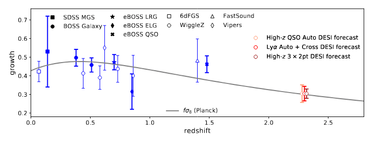
  • High-z full-shape measurement with growth rate constraints

Cuceu et al. 2021

\begin{aligned} P^{1-\operatorname{loop}}(k, \mu) & =\left(b_1-b_\eta f \mu^2\right)^2 P_{\operatorname{lin}}(k) \\ & +2 \int_{\mathbf{q}} K_2^2(\mathbf{q}, \mathbf{k}-\mathbf{q}) P_{\operatorname{lin}}(|\mathbf{k}-\mathbf{q}|) P_{\operatorname{lin}}(q) \\ & +6 K_1(\mathbf{k}) P_{\operatorname{lin}}(k) \int_{\mathbf{q}} K_3(\mathbf{k},-\mathbf{q}, \mathbf{q}) P_{\operatorname{lin}}(q) \\ & -2\left(c_0+c_2 \mu^2+c_4 \mu^4\right) k^2 P_{\operatorname{lin}}(k) . \end{aligned}
  • New EFT models for exact treatment of non-linear clustering corrections

\begin{aligned} & \tilde{K}_1(\mathbf{k})=\left(-\tau_0 b_1^\tau\right)+\left(-\tau_0\right) f \mu^2 \\ & \tilde{K}_2\left(\mathbf{k}_1, \mathbf{k}_2\right)=\frac{\left(-\tau_0 b_2^\tau\right)}{2}+\left(-\tau_0 b_{\mathcal{G}_2}^\tau\right)\left(\frac{\left(\mathbf{k}_1 \cdot \mathbf{k}_2\right)^2}{k_1^2 k_2^2}-1\right)+\left(-\tau_0 b_1^\tau\right) F_2\left(\mathbf{k}_1, \mathbf{k}_2\right)-\tau_0 f \mu^2 G_2\left(\mathbf{k}_1, \mathbf{k}_2\right) \\ & -\tau_0 \frac{f \mu k}{2}\left(\frac{\mu_1}{k_1}\left(b_1^\tau+f \mu_2^2\right)+\frac{\mu_2}{k_2}\left(b_1^\tau+f \mu_1^2\right)\right)+\frac{\tau_0^2}{2}\left(\left(b_1^\tau\right)^2+b_1^\tau f\left(\mu_1^2+\mu_2^2\right)+f^2 \mu_1^2 \mu_2^2\right) \\ & \tilde{K}_3\left(\mathbf{k}_1, \mathbf{k}_2, \mathbf{k}_3\right)=-\tau_0 Z_3\left(\mathbf{q}_1, \mathbf{q}_2, \mathbf{q}_3\right)+\tau_0^2\left[Z_2\left(\mathbf{q}_1, \mathbf{q}_2\right) Z_1\left(\mathbf{q}_3\right)\right]_{\text {symm. }}-\frac{\tau_0^3}{3!} Z_1\left(\mathbf{q}_1\right) Z_1\left(\mathbf{q}_2\right) Z_1\left(\mathbf{q}_3\right) \end{aligned}

Ivanov 2024

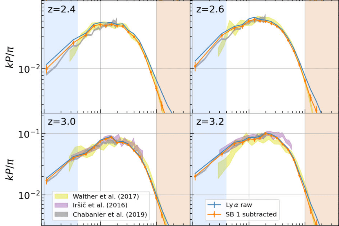
P1D measurements on high resolution

  • KODIAQ + SQUAD + XQ-100 measurement
  • Very few quasars (538)
  • Goes to very small scales = more constraining power for dark matter models

Karacaylı et al. 2022
P1D

Wavenumber k [s/km]

eBOSS constraints

Palanque-Delabrouille et al. 2020
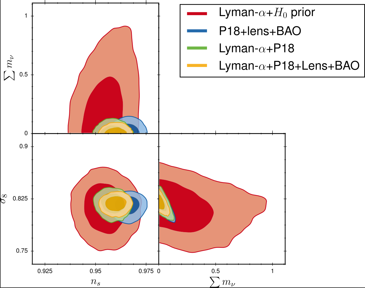
  • Neutrino mass  (P1D +CMB):
\sum m_{\nu} < 0.11~\mathrm{eV}
m_{\mathrm{X}} > 5.3~\mathrm{keV}
  • Warm dark matter model:
  • Other constraints: Fuzzy dark matter, sterile neutrinos, running of the primordial power spectrum

at 95% C.L.

at 95% C.L.
Slide taken from Jonas Chaves-Montero (Moriond 2026)