Growth rate from SNIa peculiar velocity and galaxy density field
Corentin Ravoux - CNRS/LPCA Clermont-Ferrand



ACCEL² simulation
with Bastien Carreres, Julian Bautista, Damiano Rosselli and many others
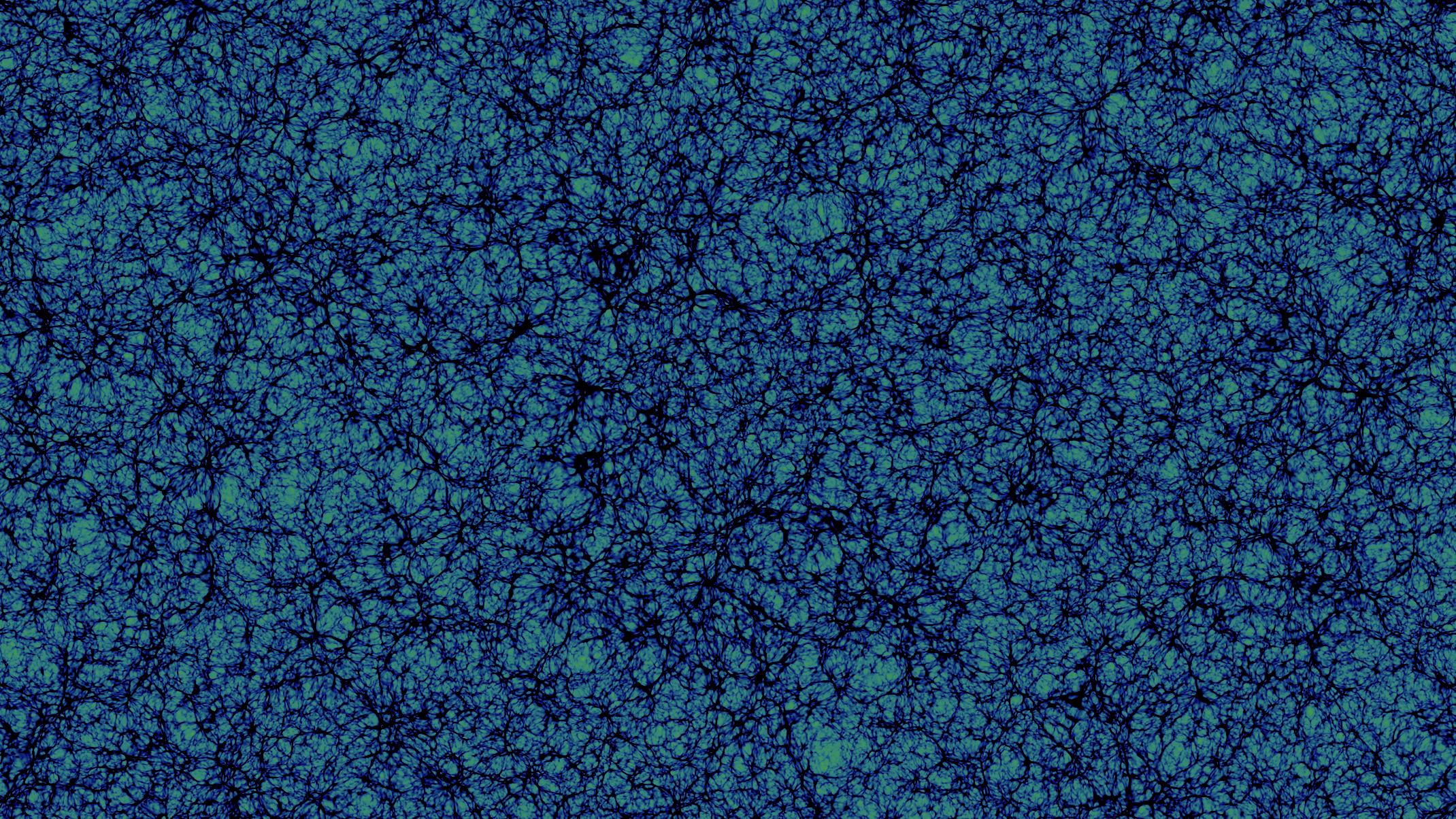

Measuring fσ8
Peculiar velocities (PV)
Redshift Space Distortions (RSD)
- Direct estimation of velocities
- Need an estimate of redshift ( ) and distance (decoupling from )
- Compute statistics from PV
- Impact of PV on measurements
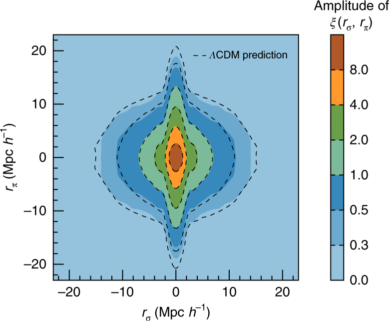
- Example: galaxy auto-correlation, void cross-correlation, ...
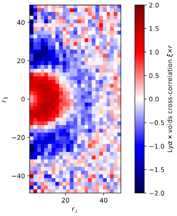
Ravoux et al. 2022
He et al. 2018
Corentin Ravoux DESI presentation - June 26
fσ8 constraints
- Constrain modified gravity models
- RSD very effective for high redshift
- PV for low redshift
- Improvement with method combination
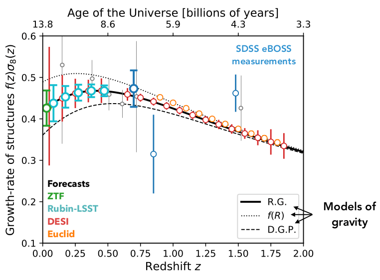
from Julian Bautista
Corentin Ravoux DESI presentation - June 26
Type Ia supernovae
- Distance modulus:
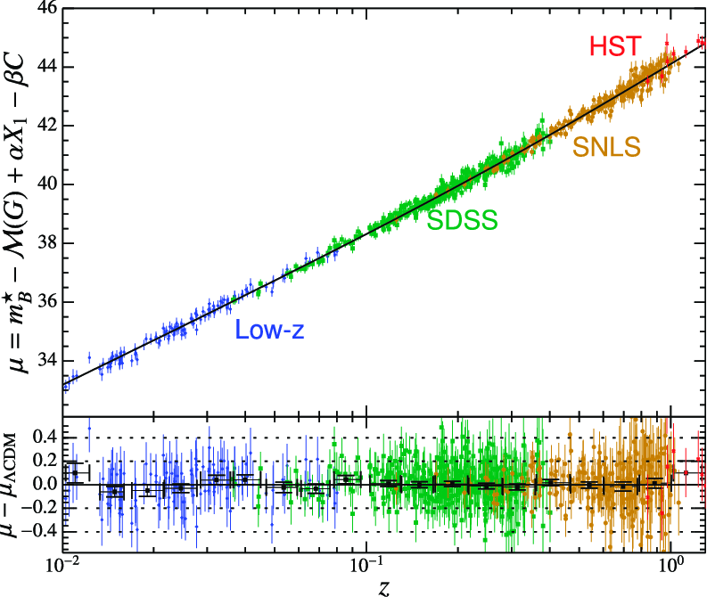
Betoule et al. 2014
- SNe Ia standardization = Tripp relation
Light-curve stretch
SN color
Parameters common for all SN Ia
"Redder is fainter"
"Luminous fade slowly"
- SNe Ia: Thermonuclear explosion a white dwarf reaching Chandrasekhar mass
Corentin Ravoux DESI presentation - June 26
Type Ia supernovae
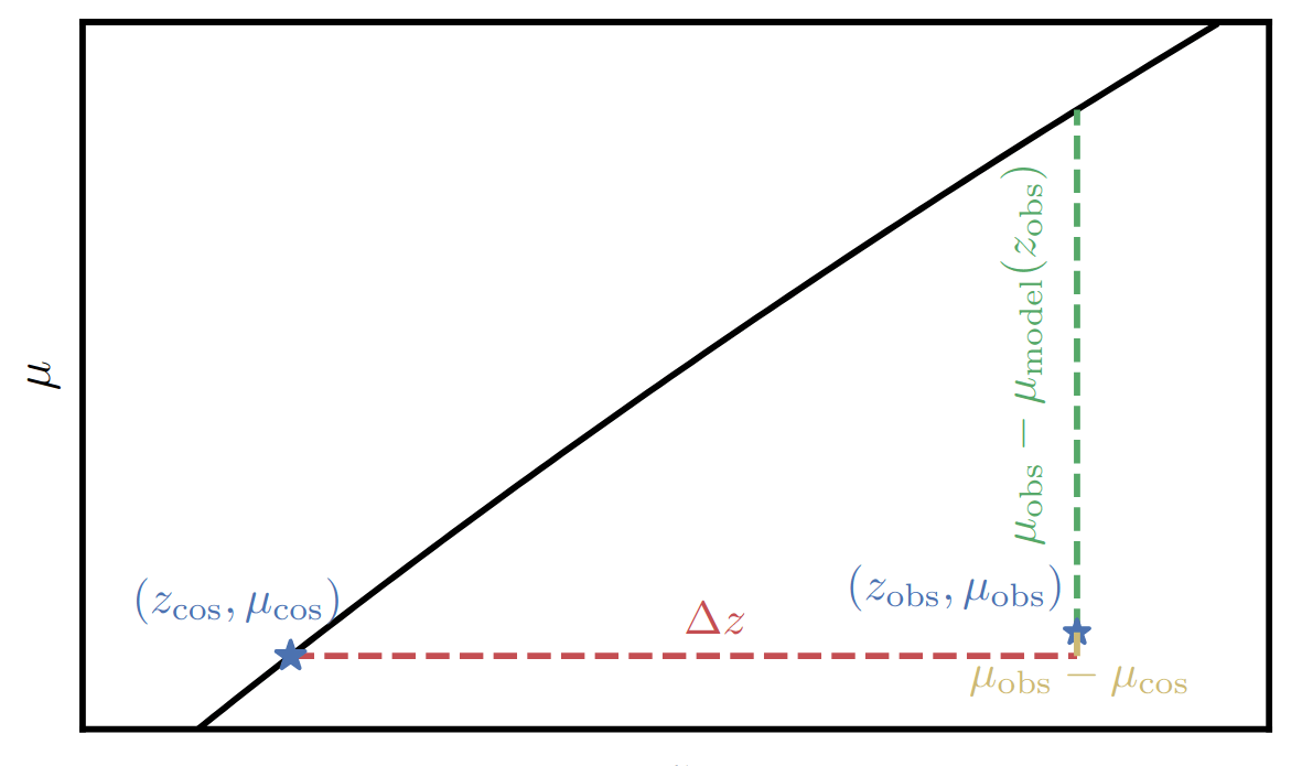
- Hubble residuals:
- Velocity estimator:
Carreres et al. 2023
Corentin Ravoux DESI presentation - June 26
Likelihood-based field-level inference
ACCEL² simulation
ACCEL² simulation
Carreres et al. 2023
Ravoux et al. 2025
Corentin Ravoux DESI presentation - June 26
Likelihood-based field-level estimator
Velocity from SNe Ia
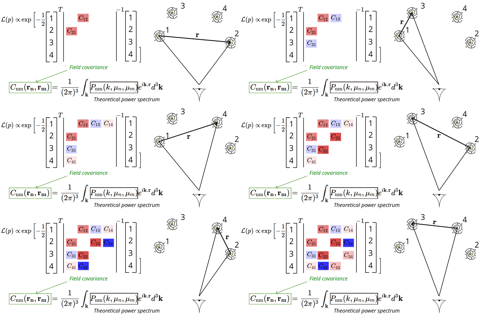
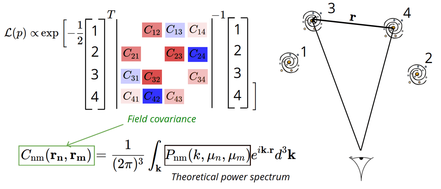
Field covariance matrix computed from theory and coordinates
Parameters
Velocity example:
- Purpose: Maximizing or sampling a likelihood computed from all coordinates of the data
- p = fitted parameters: simultaneously cosmology (fσ8) and field parameters (e.g., Hubble diagram parameters α, β, M0 for SN)
Corentin Ravoux DESI presentation - June 26
Computing the field covariance
Corentin Ravoux DESI presentation - June 26
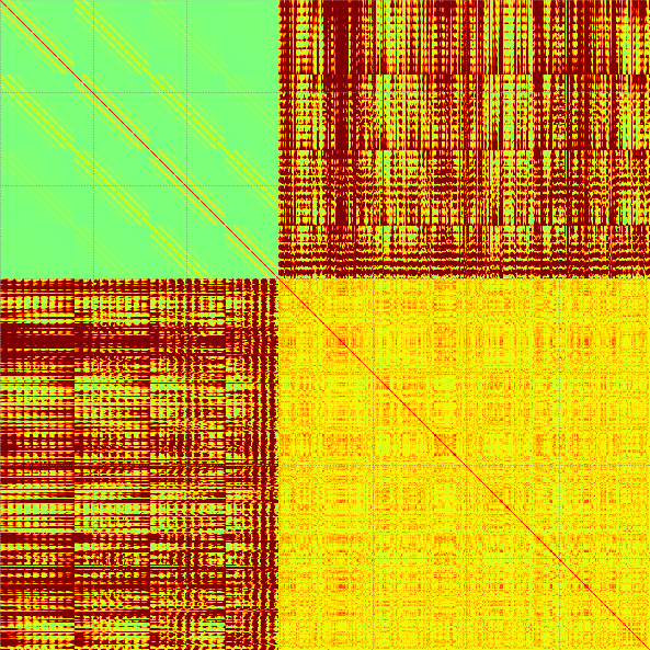
Combining densities (RSD) and peculiar velocities
Velocities
Density field from galaxy surveys
Full field covariance matrix
Corentin Ravoux DESI presentation - June 26
General covariance calculation
- Objective: Improve/Extend the likelihood-based modeling
- General form of field power spectrum
- Algorithmically-oriented calculations (Hankel transforms)
- Wide-angle effect accounted in the integration
gg, gv, vv
Parameters to fit
Terms to integrate analytically
Power spectra terms to integrate numerically
Corentin Ravoux DESI presentation - June 26
flip Field Level Inference Package
- python package for likelihood-based field-level inference:
https://github.com/corentinravoux/flip
- Fast generation of field covariance
- Symbolic code generation for covariance model
- MCMC and Minuit to fit fσ8
- General expression for vectors (SNIa, density, log distance, TF, FP...)
- Survey geometry-dependent Fisher forecast
Contributors: Bastien Carreres, Damiano Rosselli and Alex G. Kim
Flip article: arxiv:2501.16852
Corentin Ravoux DESI presentation - June 26
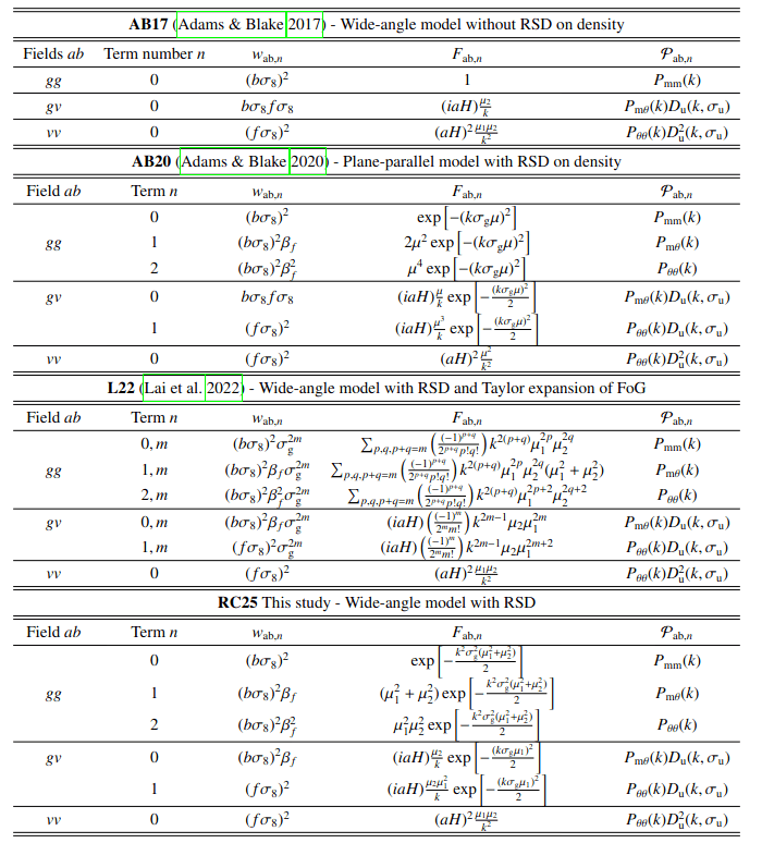
Field covariance models
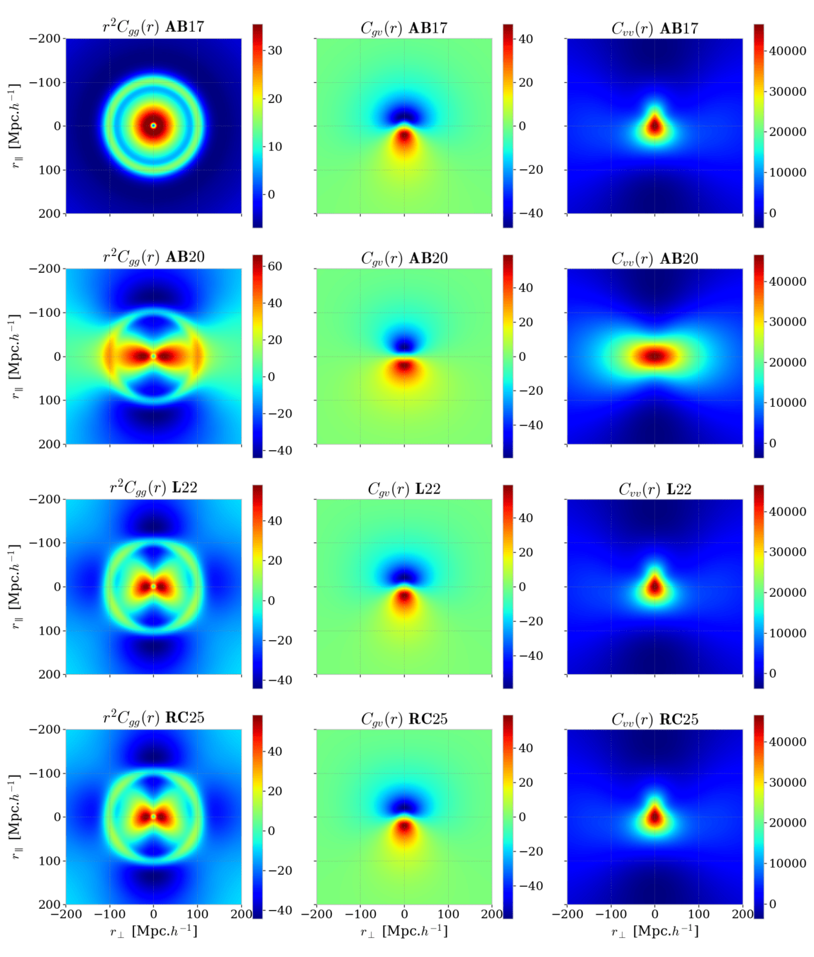
- Model comparison on a regular coordinate grid (Adams & Blake 2017, Adams & Blake 2020, Lai et al. 2022)
- New wide-angle model developed (RC25): improved stability in integration and for wider fitting parameter ranges
Ravoux et al. 2025
Corentin Ravoux DESI presentation - June 26
Combining DESI galaxy density and ZTF SNIa velocities on simulation
ACCEL² simulation
ACCEL² simulation
Ravoux et al. in prep
Corentin Ravoux DESI presentation - June 26
ACCEL² simulation
Zwicky Transient Facility (ZTF)
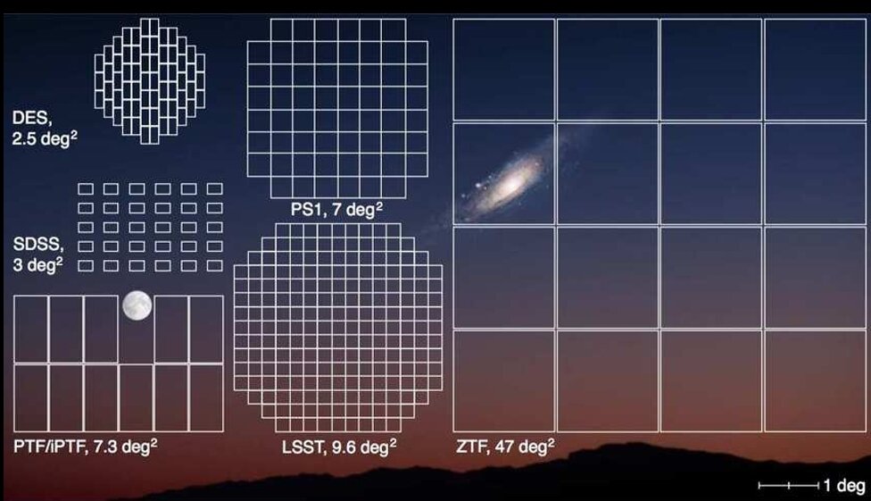
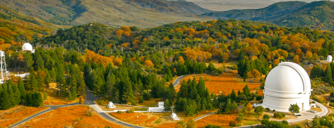
- ZTF = high-cadence photometric telescop in the Palomar observatory
- Very large field of view (47 deg²)
- Observing 3/4 of the sky every nights with 3 filters (g, r, i)
- Transient sky: Supernovae, gamma ray burst, tidal distruptive events, comets, asteroids
-
Dedicated spectroscopic telescope measuring transient spectra (SEDmachine)
Corentin Ravoux DESI presentation - June 26
SN Ia simulation and analysis

SN Ia simulator
Survey parameters
SN Ia model
N-body host simulation
Realistic SN Ia light curves
Quality cuts
(Detection, spec-z selection, light curve quality...)
Light curve fit (SALT2)
Velocity estimation and simultaneous fit of fσ8 and velocity parameters
Simulation
Analysis
Corentin Ravoux DESI presentation - June 26
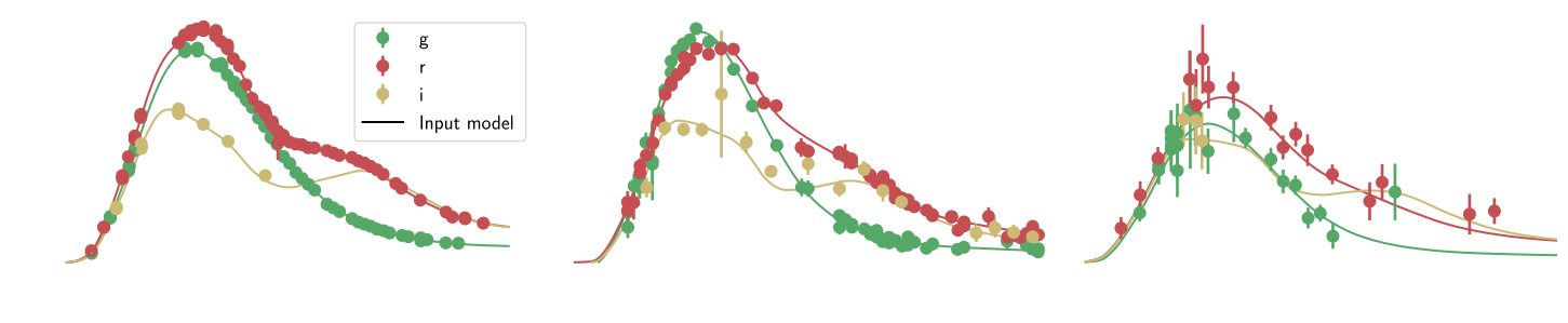
snsim
https://github.com/bastiencarreres/snsim
- Survey parameters: Cadence (ZTF, LSST), CCD gain, zero point, sky noise
- SN Ia model: Rate, SED, color, stretch, intrinsic scattering distributions, light-curve parameters
- Host catalog: Use velocities and associated clustering from N-body simulation
Flux
Phase
Phase
Phase
Carreres et al. 2023
Main contributors: Bastien Carreres, Damiano Rosselli
Corentin Ravoux DESI presentation - June 26
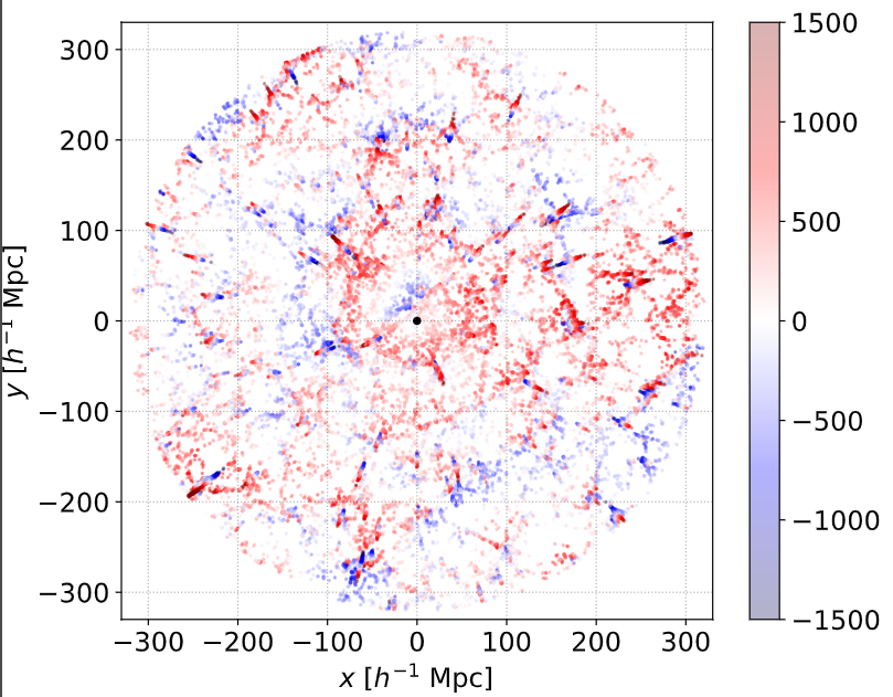
DESI x ZTF simulation
- 27 simulations from AbacusSummit (Maksimova et al. 2019)
- Density: DESI Bright Galaxy Survey (BGS) clustering matching for DR3 (J. Bautista, A. Smith)
- Velocity: ZTF SNIa Y6 simulation performed (following Carreres et al. 2023)
from Julian Bautista
Corentin Ravoux DESI presentation - June 26
Galaxy field
Supernovae velocities
- Runs of SNsim to mimic ZTF SNIa Y6 data set (following Carreres et al. 2023)
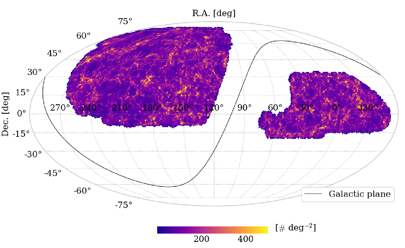
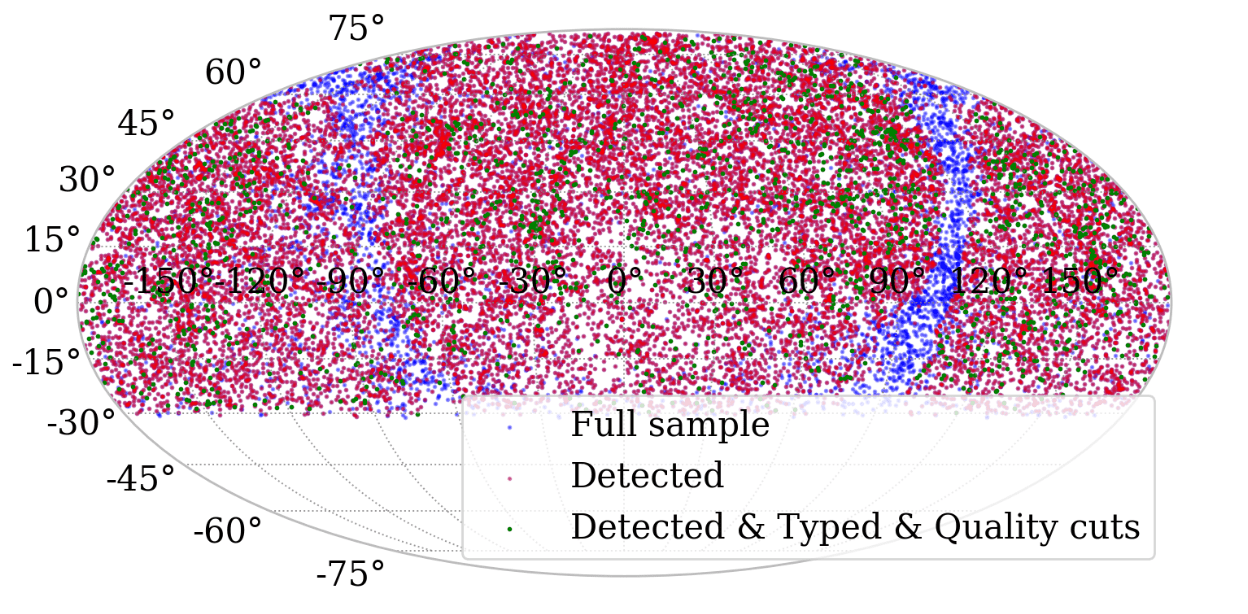
- AbacusSummit mocks matching DESI DR3 (5 years) BGS clustering and footprint
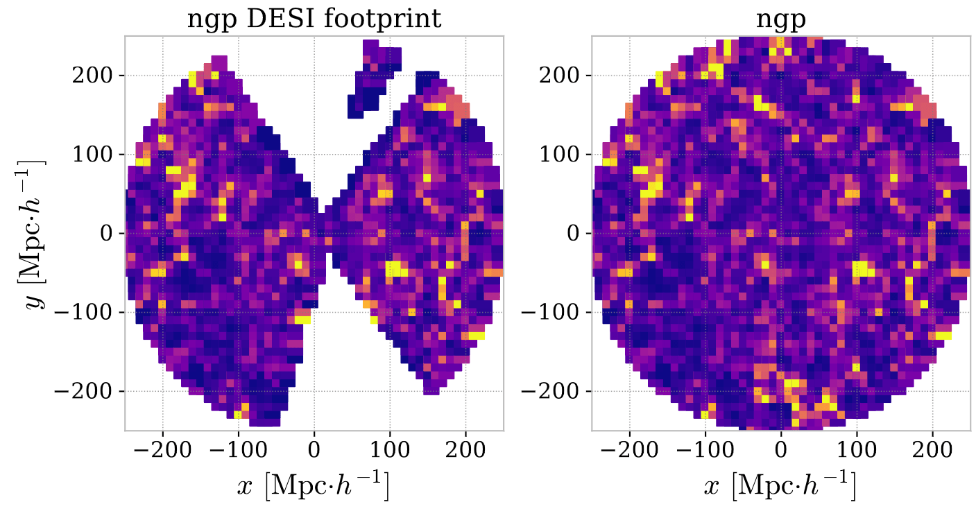
Ravoux et al. in prep.
Corentin Ravoux DESI presentation - June 26
Model for density & velocity fit
- Use of the RC25 wide-angle model implemented in flip:
Corentin Ravoux DESI presentation - June 26
ZTF velocity fit
- Velocity fit including Hubble diagram parameters to reproduce Carreres et al. 2023
- Variation of analysis parameters (max redshift, SNIa density...)
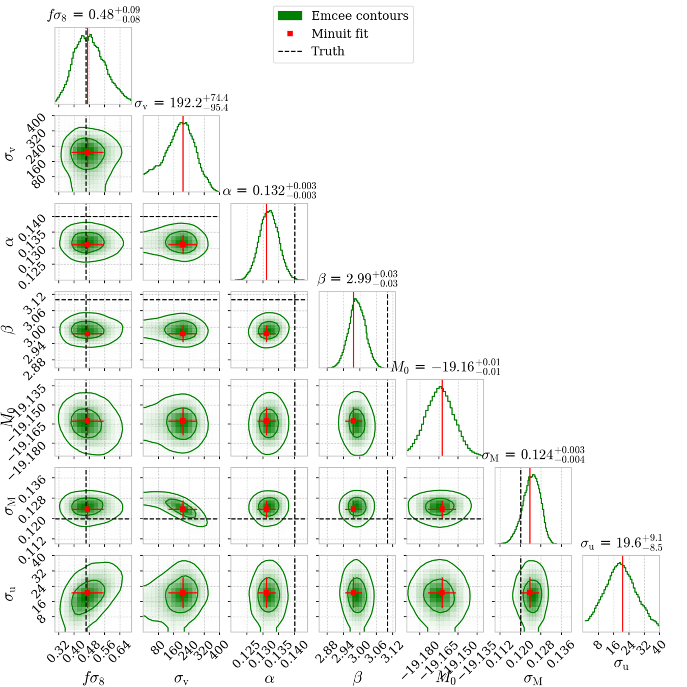
Ravoux et al. in prep.
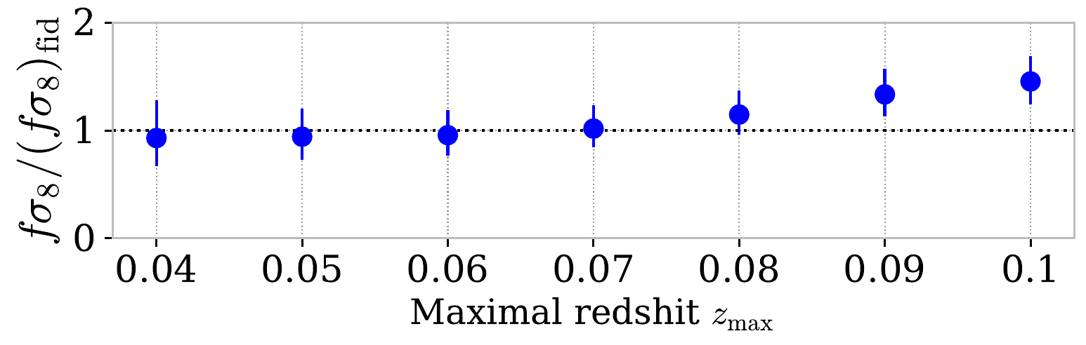
Corentin Ravoux DESI presentation - June 26
DESI density fit
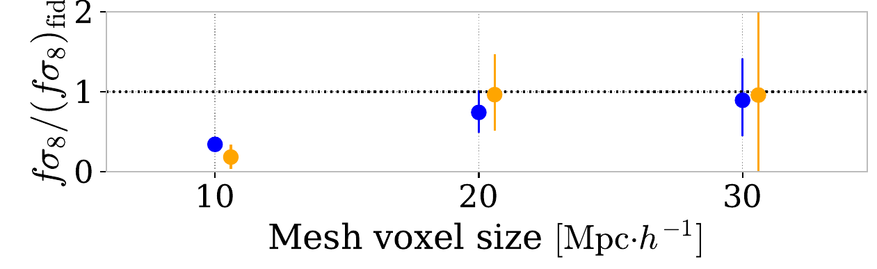
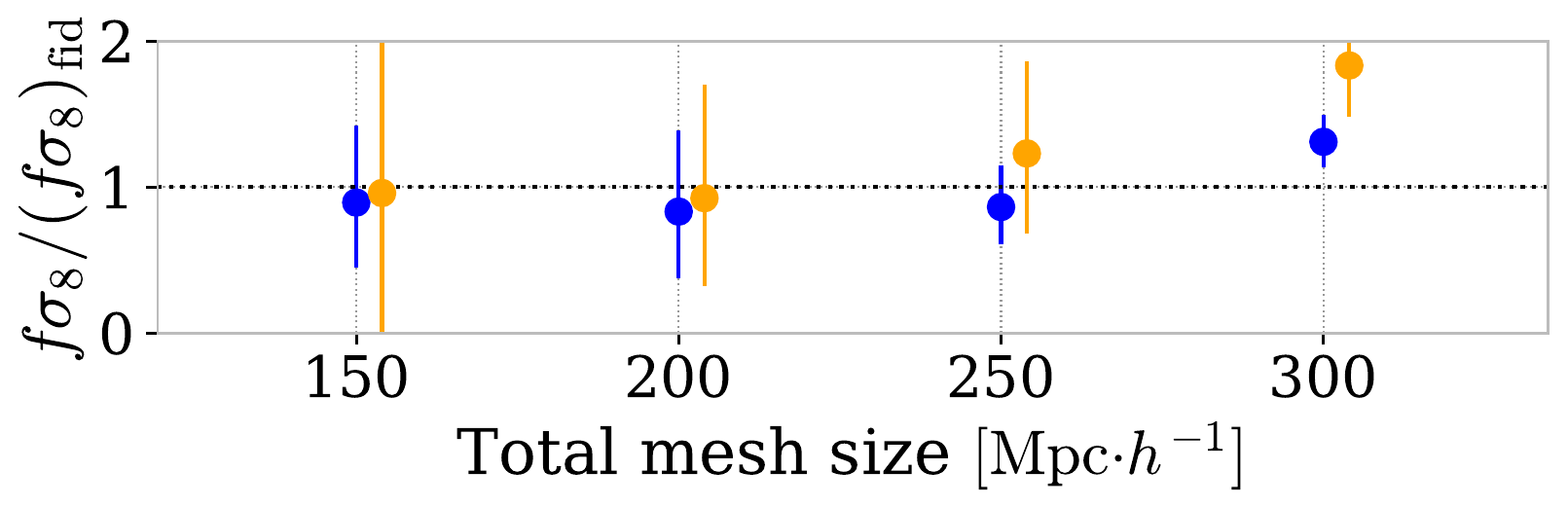
- Density grid with pypower
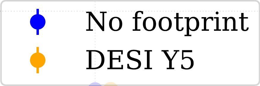
- Test varying all density gridding parameters: grid size, mesh cell size, interpolation scheme (NGC, CIC, TSC, PCS), footprint (DESI DR3 or no cut)
- Mean minuit fit on 27 mocks with average error bar
Ravoux et al. in prep.
Corentin Ravoux DESI presentation - June 26
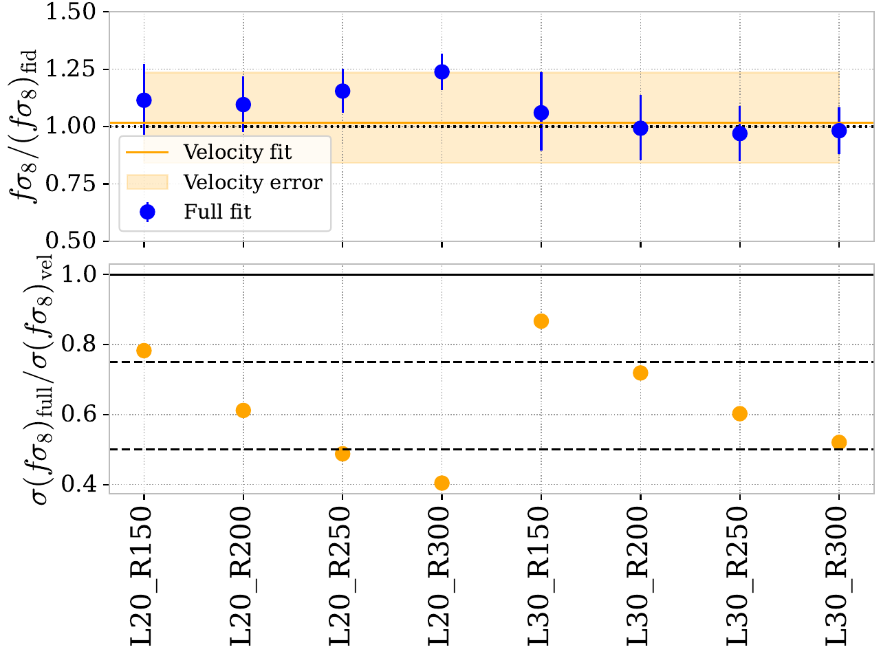
DESI x ZTF joint fit
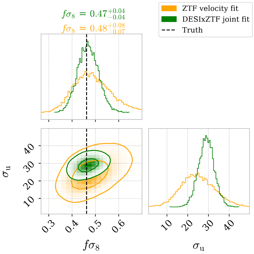
- SNIa velocity fit with Hubble diagram parameters and density field
Adding density improves fs8 constraints up to 50%
Different density configurations
Ravoux et al. in prep.
Corentin Ravoux DESI presentation - June 26
Summary of PV estimations on realistic simulations
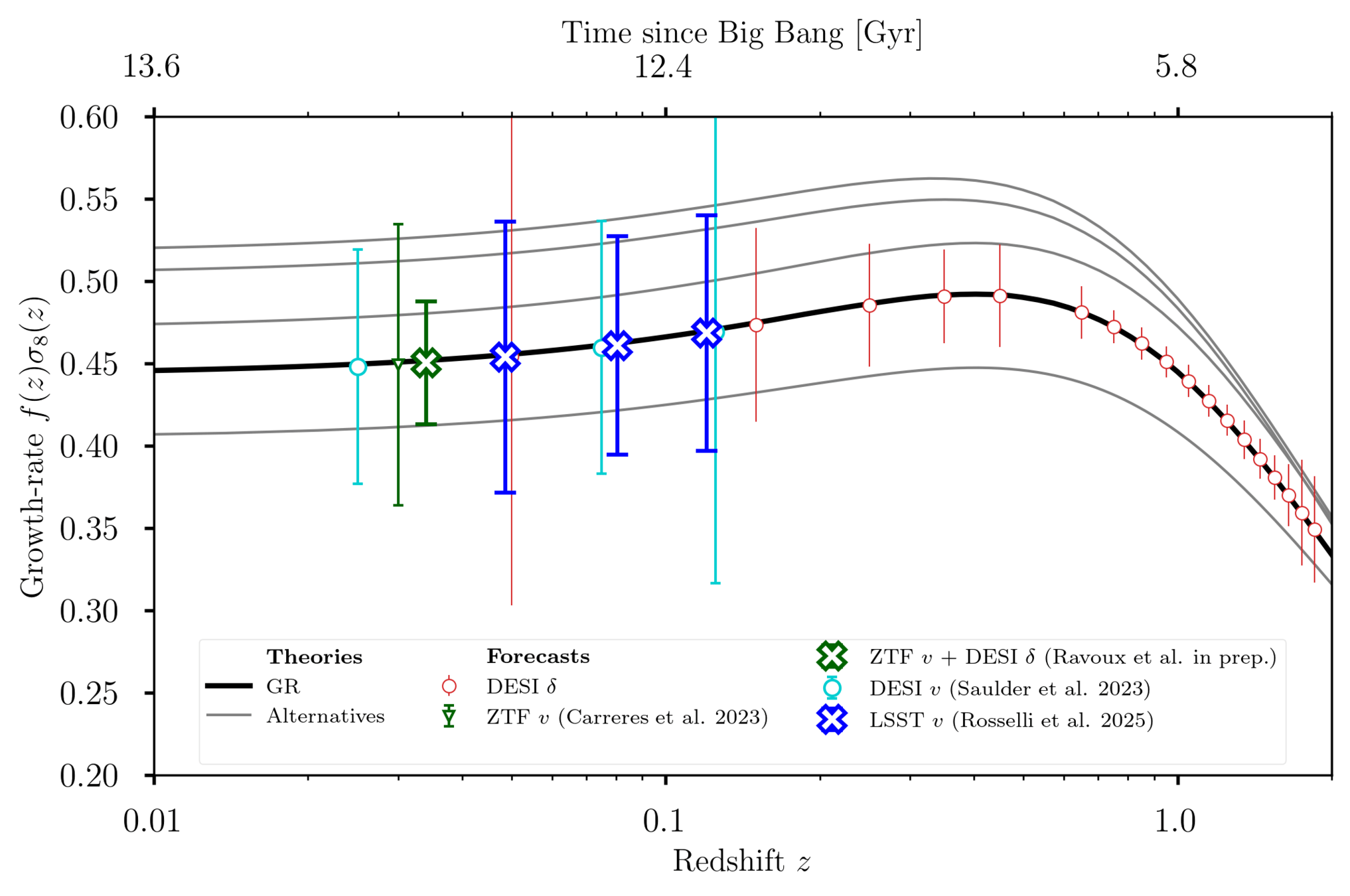
ZTF + DESI
(this talk)
ZTF (Carreres et al. 2023)
LSST (Rosselli et al. 2025)
Corentin Ravoux DESI presentation - June 26
Conclusion
- Large modeling and simulation preparatory work for ZTF, LSST and combination with DESI density field
- Dedicated sofware for simulation (snsim, skysurvey) and analysis (flip)
- DESI ZTF simulation article draft ready
ACCEL² simulation
Hubble diagram
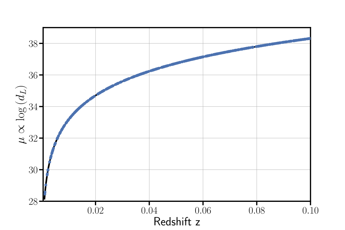
Perfect standard candle in an expanding Universe
from Bastien Carreres
Standard candle = object with fixed luminosity
Hubble diagram
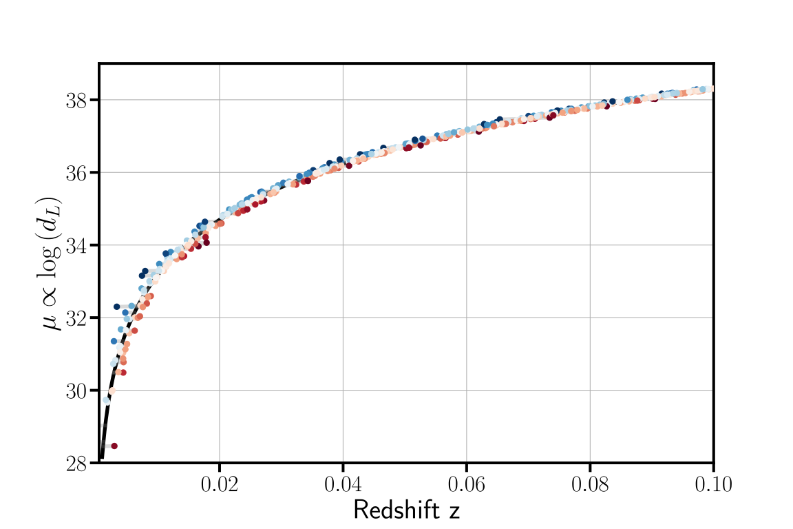
Peculiar velocities
from Bastien Carreres
Perfect standard candle in an expanding Universe
Hubble diagram
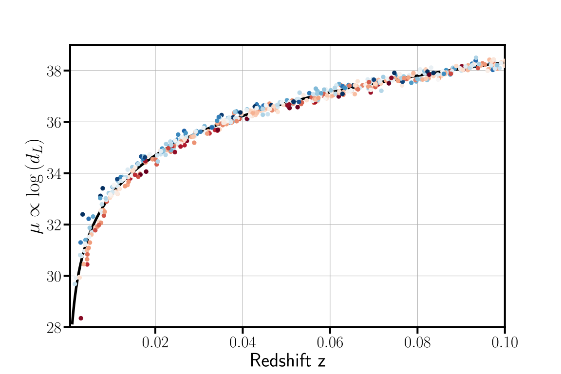
Noise sources (intrinsic scatter, local environment, instruments...)
from Bastien Carreres
Standardizable candle in an expanding Universe
Peculiar velocities
Hubble diagram
from Bastien Carreres
High redshifts = dark energy constraints (w, or w0,wa)
Low redshifts + calibration of the candle luminosity = H0 constraints
Hubble residuals = fσ8 constraints
Dark Energy
- What is the nature of dark energy ?
- Cosmological constant model (Λ) not very satisfying
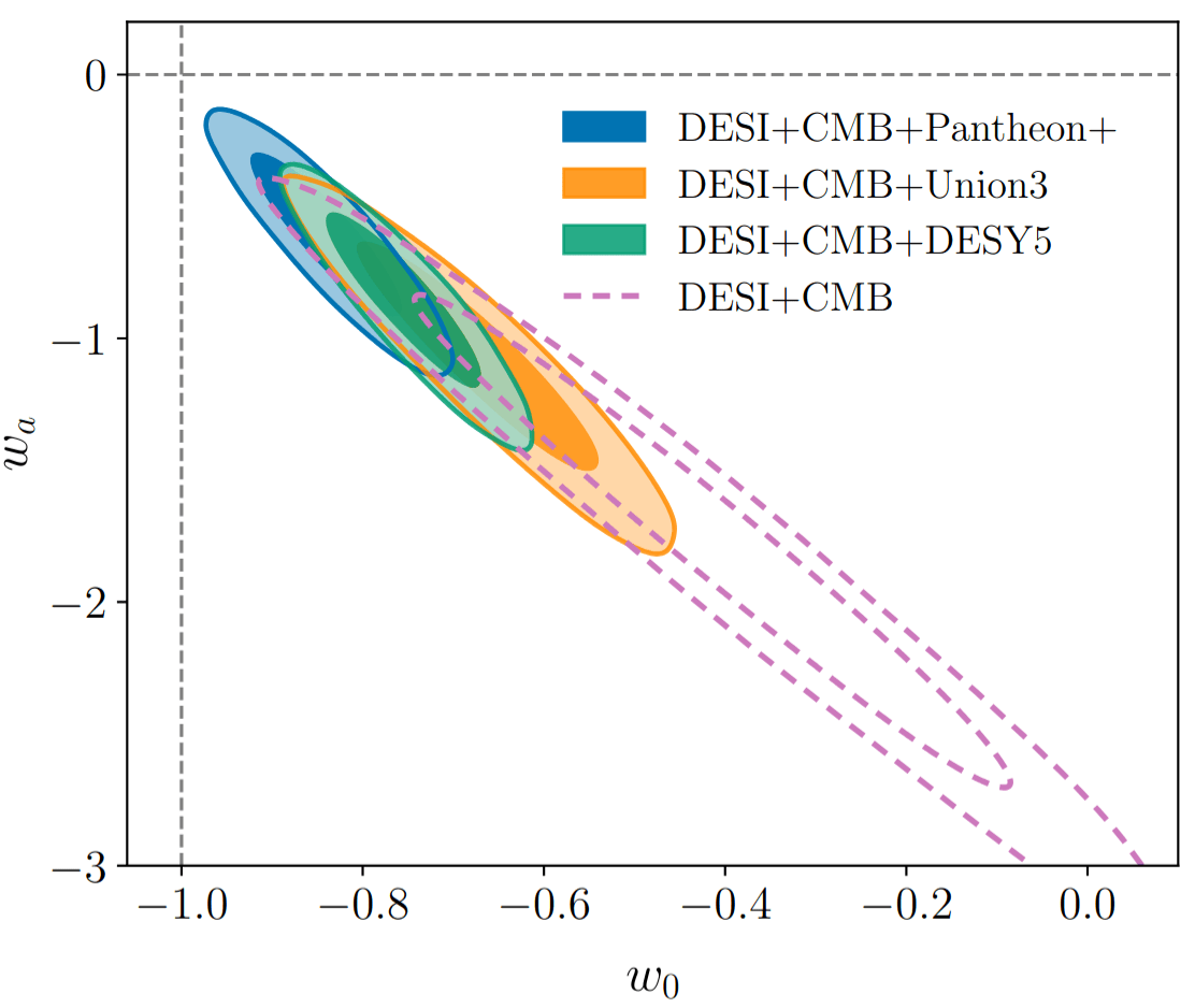
Recent DESI DR2 BAO + CMB + SNIa results: stronger hints for varying dark energy
DESI DR2 BAO 2025
Dark Energy
- What is the nature of dark energy ?
- Cosmological constant model (Λ) not very satisfying
-
Other models :
- Fifth force, additional field ?
- Modified gravity theories ?
- Our current objective: Probing large-scale structure formation to constrain dark energy/modified gravity.
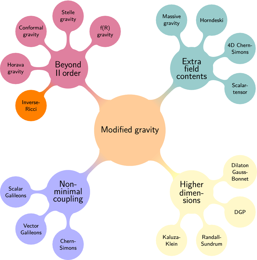
Shankaranarayanan et al. 2022
Cosmic web
- Matter perturbations in the primordial Universe grew to form the cosmic web
- Static description: matter density contrast (δ) follows a linear power spectrum at large-scales
- Dynamic description: Cosmic web peculiar velocities ( ) caused by gravitation
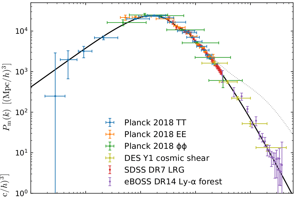

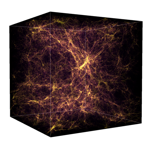
Walther et al. 2021
Chabanier et al. 2019
fσ8 parameter
- Linear perturbation theory:
Cosmic web velocities
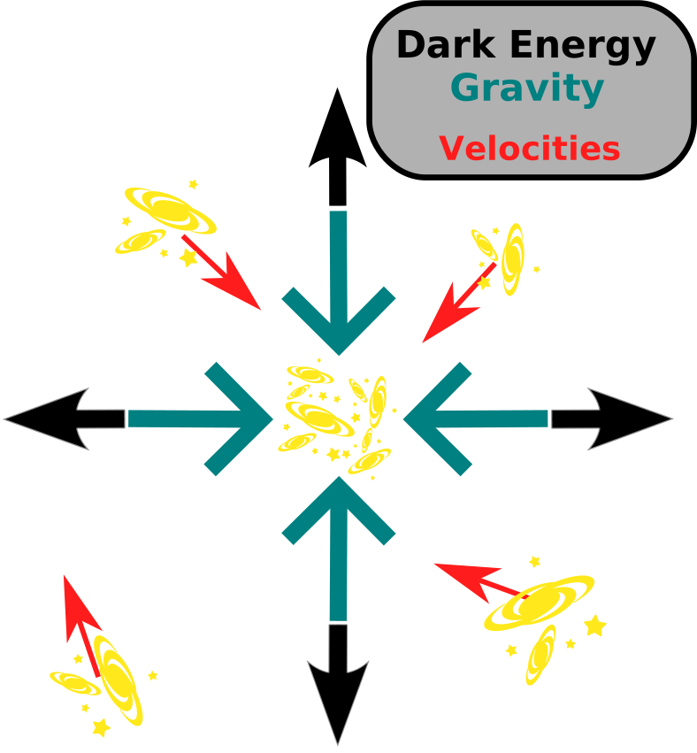
Normalized matter overdensity
fσ8 parameter
- Linear perturbation theory:
Cosmic web velocities
Normalized matter overdensity
Logarithmic growth rate of linear perturbations
8 Mpc/h
Amplitude of the matter perturbations in spheres of 8 Mpc/h comoving radius (matter power spectrum amplitude)
in GR
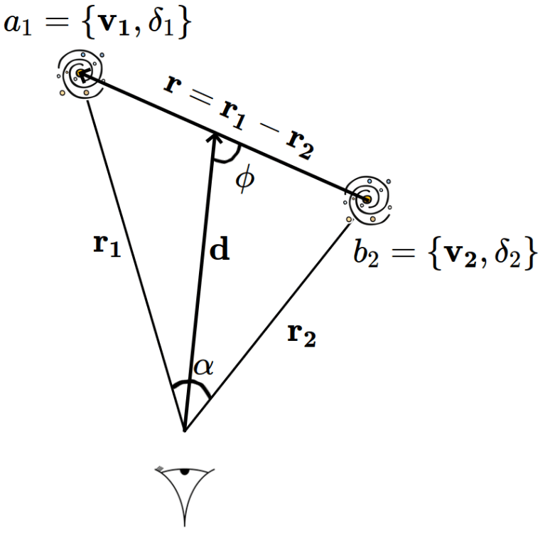
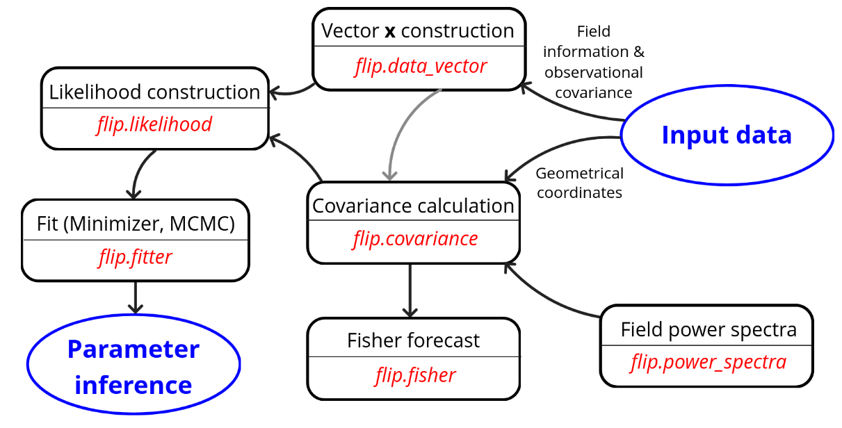
A word on wide-angle in clustering

Plane parallel models
Wide angle models
Plane parallel model
- Express power spectrum model in a general way:
- vv "simple" example:
Parameters to fit
Terms to integrate analytically
Power spectra terms to integrate numerically
Plane parallel model
- Without loosing generality we can express the covariance:
Plane parallel model
Linear sum of matrix with parameters to fit as coefficients
- Without loosing generality we can express the covariance:
Plane parallel model
Hankel transform
- Most important part: Algorithmically optimized way to compute power spectrum integral, with FFTLog algorithm
- Without loosing generality we can express the covariance:
Plane parallel model
- Without loosing generality we can express the covariance:
Terms pre-computed analytically with symbolic code generaltion
- More complicated formalism derived and implemented for wide-angle
Wide angle model
linear sum of matrix
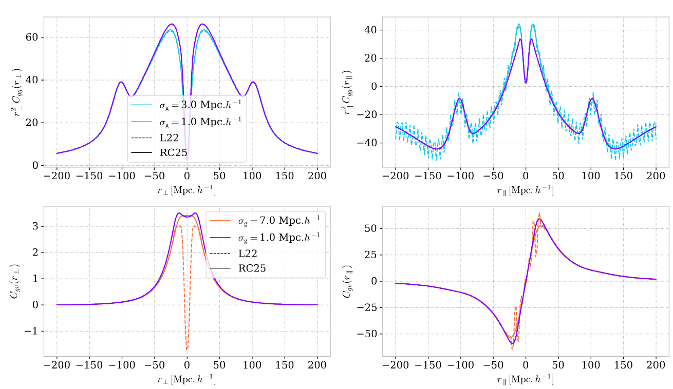
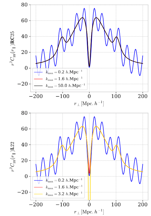
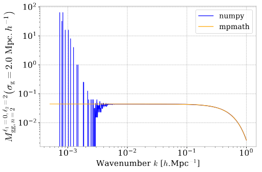
flip validations
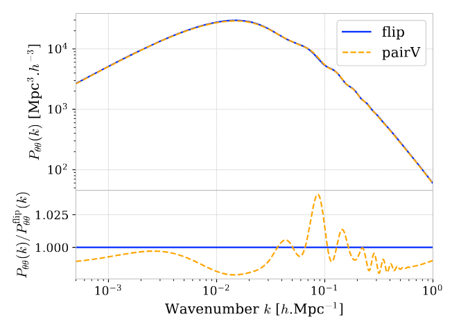
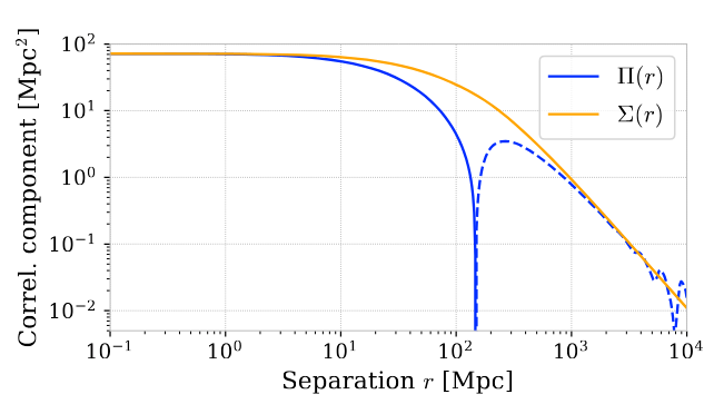
- Field covariance comparison with pairV Anthony Carr & David Parkinson
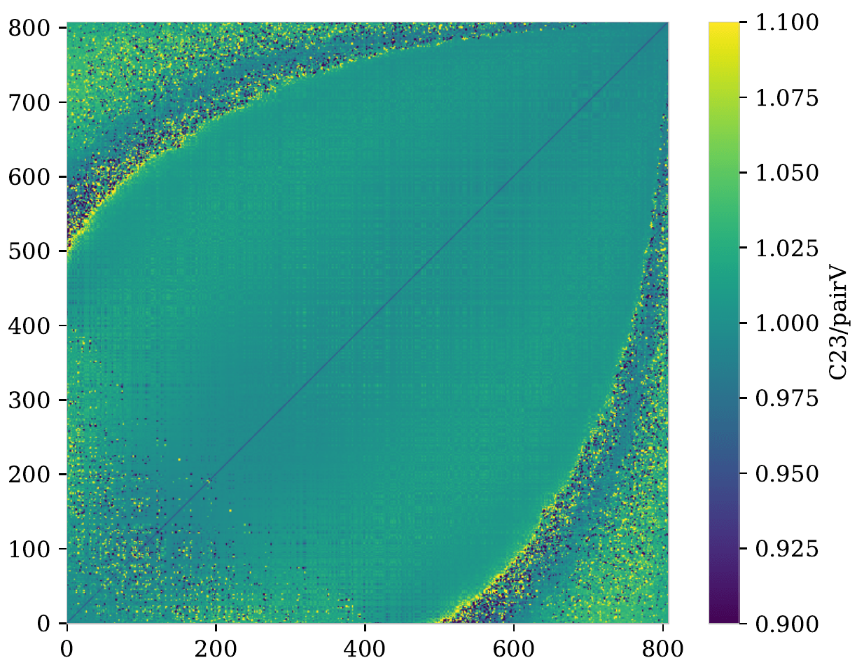
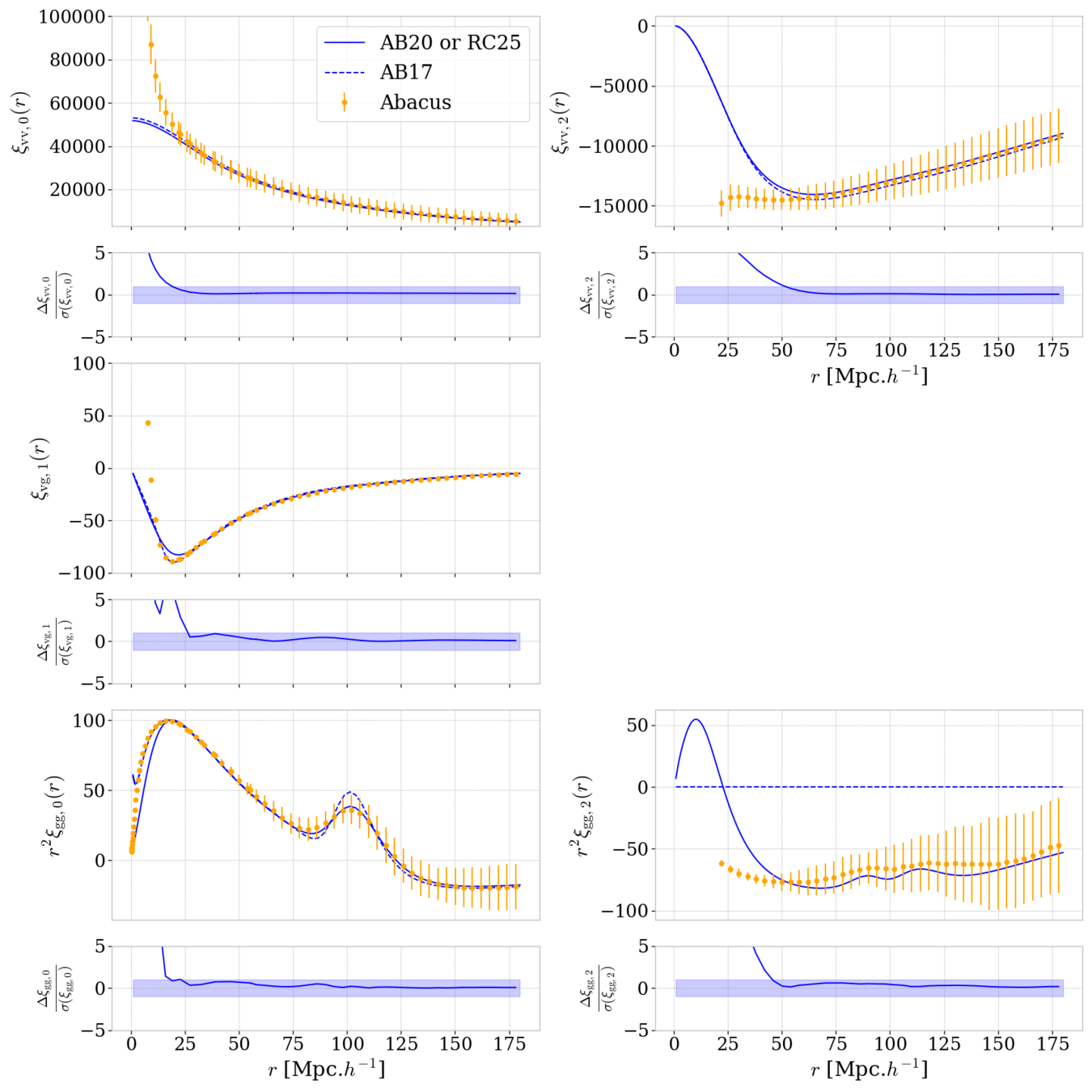
- Model validated on N-body simulations Tyann Dummerchat
Disagreement due to different power spectrum model
Ravoux et al. 2025
Ravoux et al. 2025
Survey dependent Fisher forecast
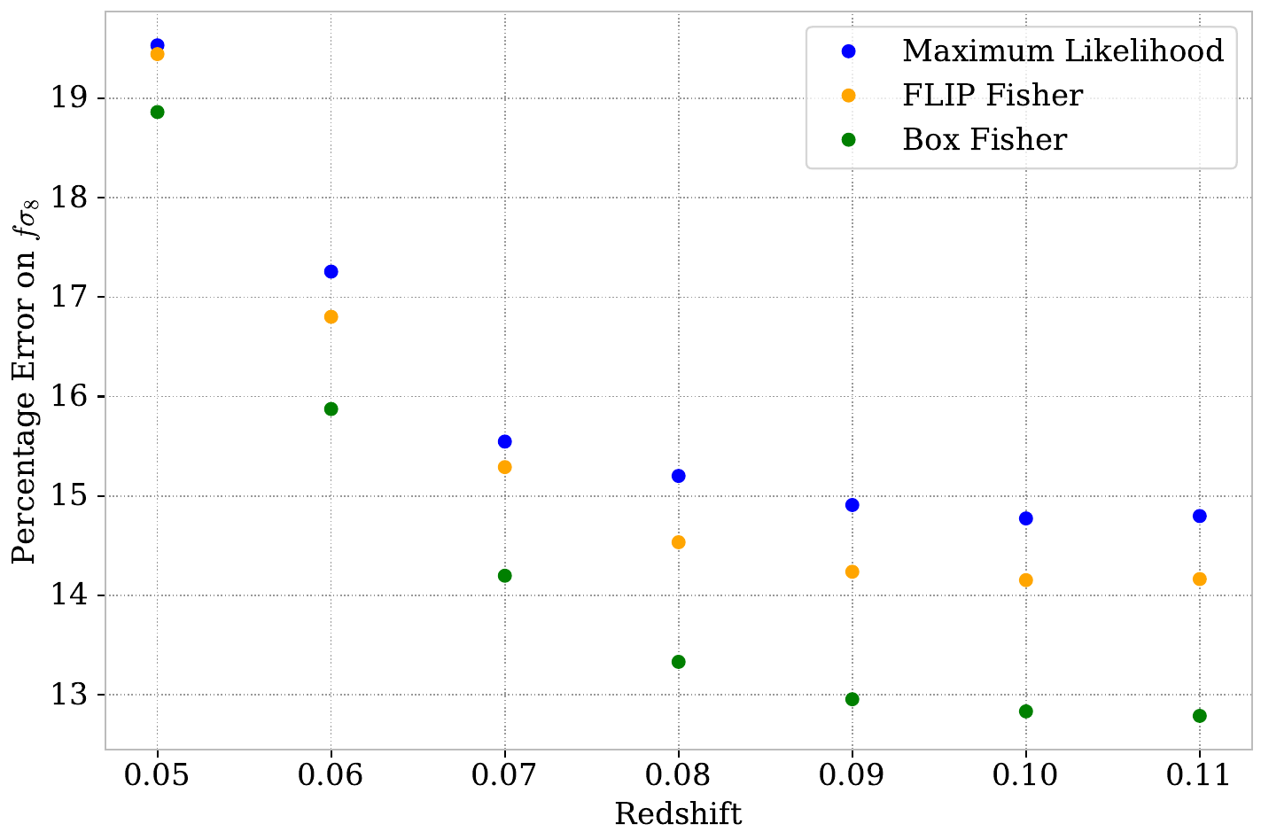
- Field covariance matrix accounts for survey geometry
- Comparing ZTF simulation (Carreres et al. 2023) with Fisher forecasts
- Error ~ 30% closer to likelihood-based than standard Fisher
Howlett et al. 2017
Ravoux et al. 2025
Rubin - LSST
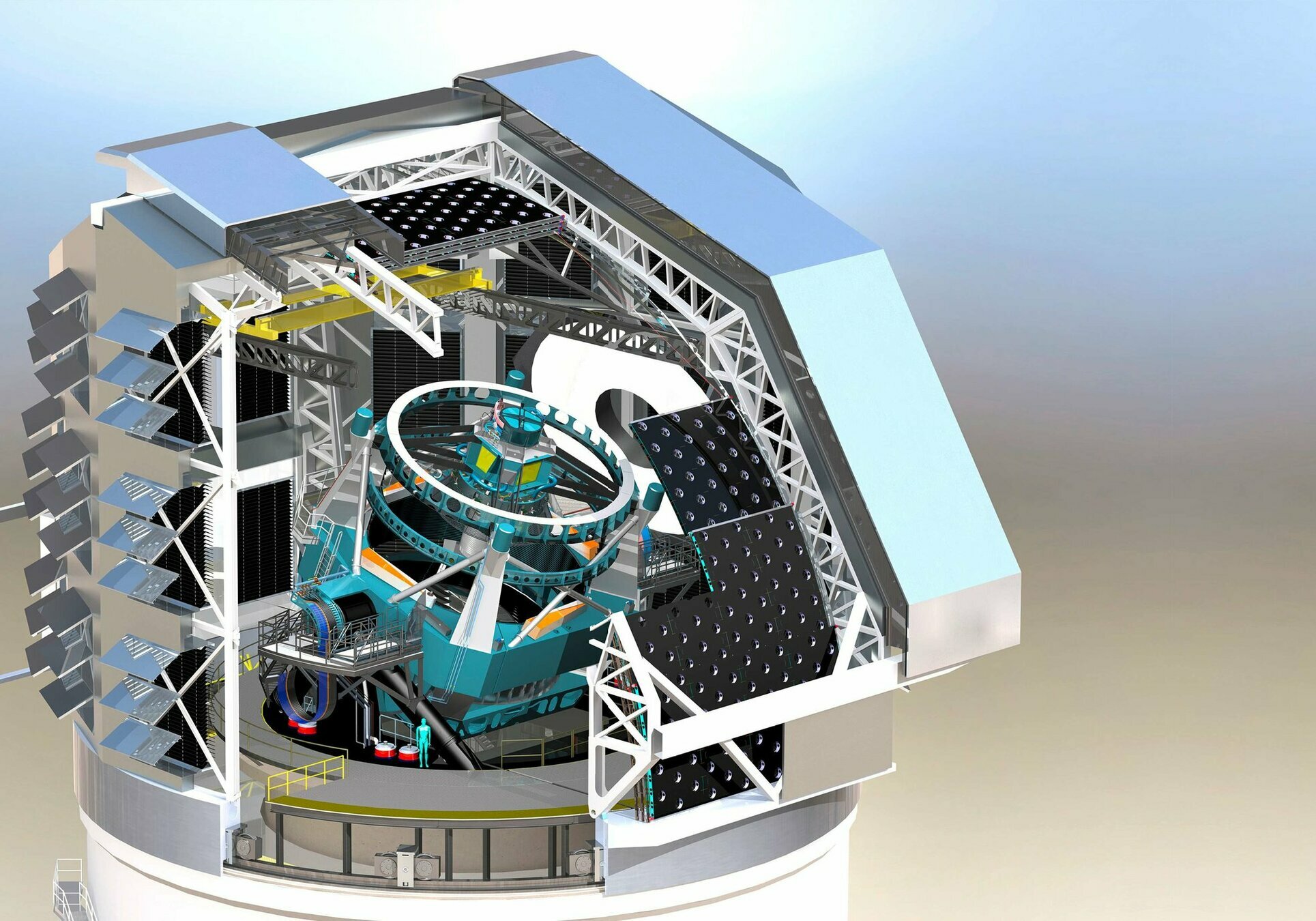
Telescope mount assembly
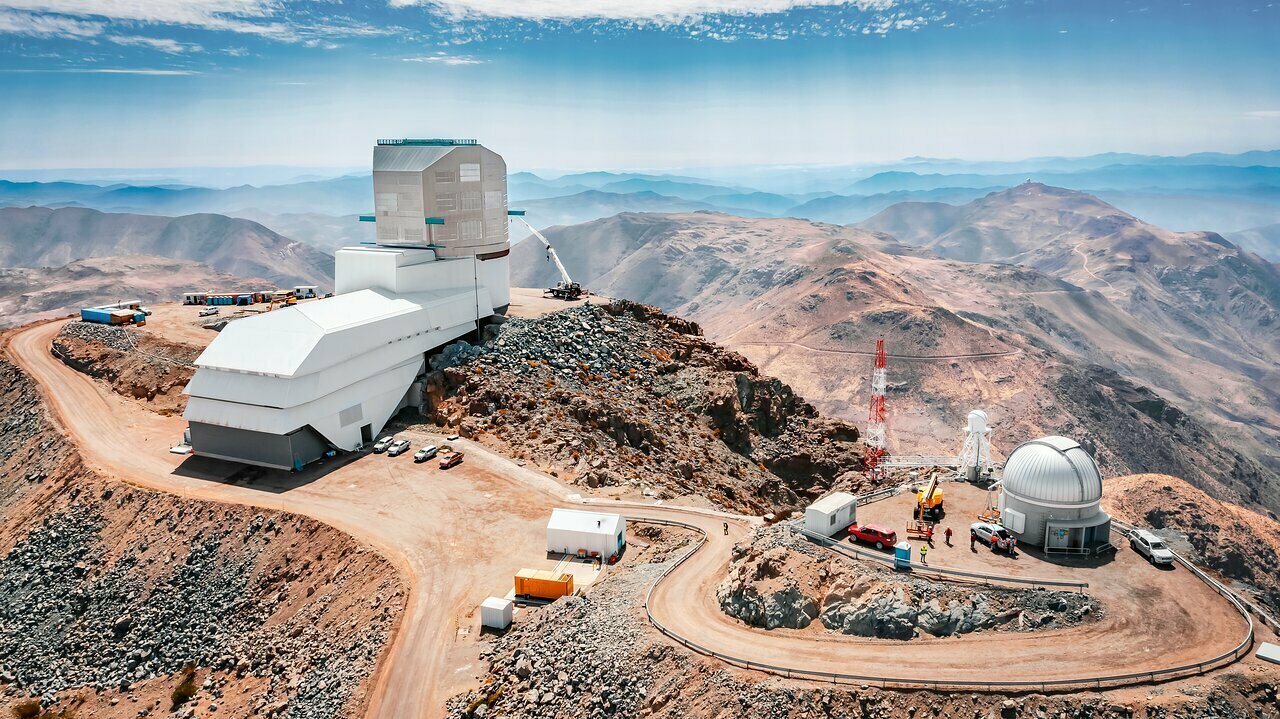
AuxTel: 1.2m atmospheric telescop
Rubin - LSST: instrument
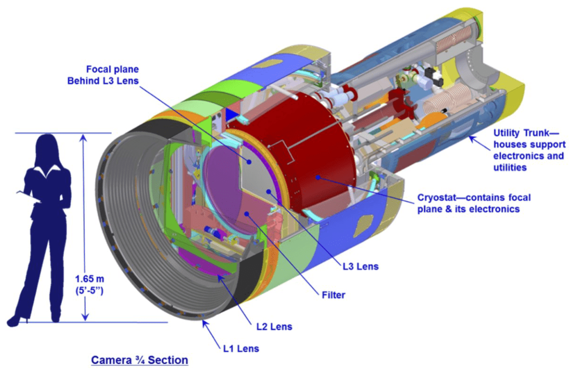
- Largest numerical camera in the world: 3.2 Gpixels with 2s readout time
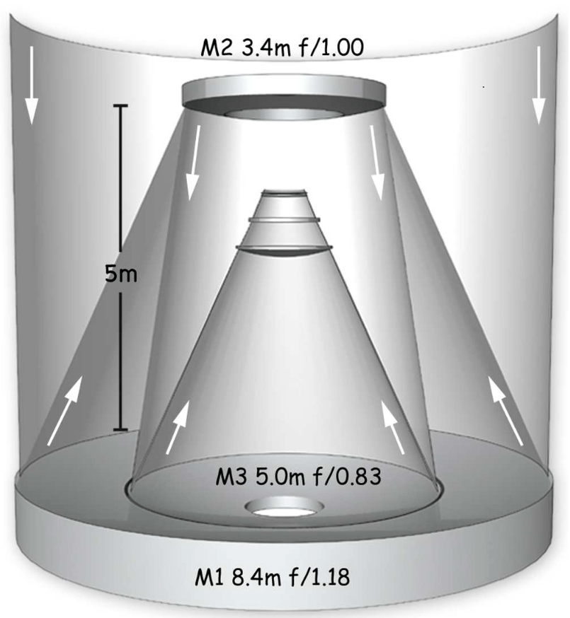
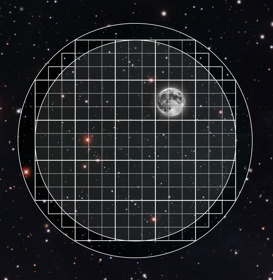
- 8.4 m primary mirror and 9.6 deg² field of view
- 6 filters: (u, g, r, i, z, y)
- 10-year photometric survey of half of the sky (~ 20 000 deg²)
ZTF results
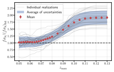
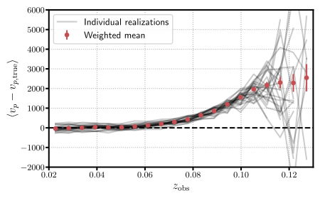
- SN Ia selection bias causes velocity & fσ8 bias at high redshift
- No fσ8 error bar improvement even with correction
- Maximum redshift usable:
Carreres et al. 2023
Carreres et al. 2023
ZTF results
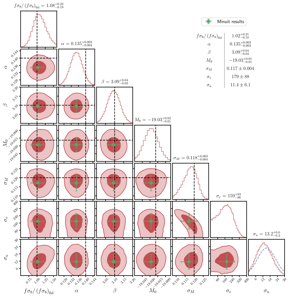
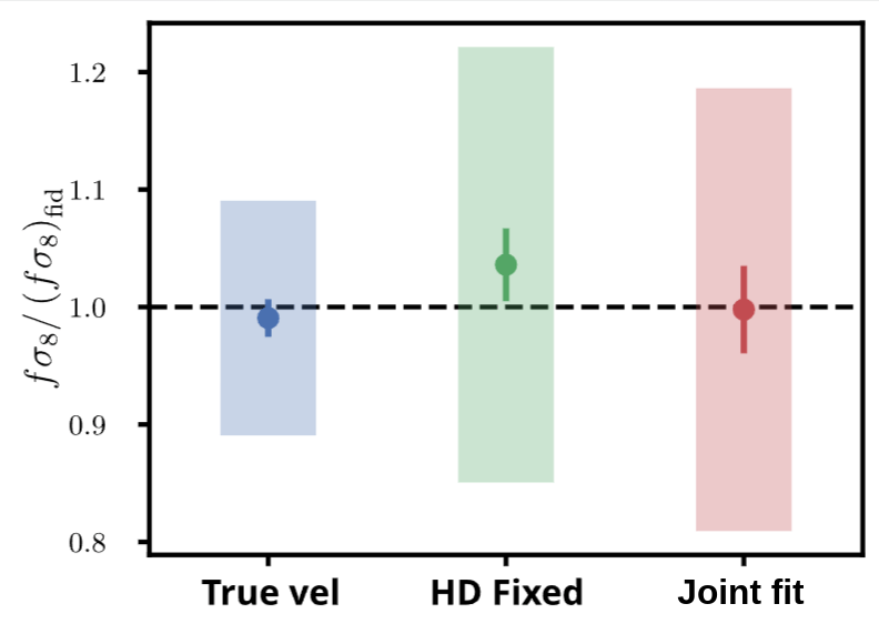
- fσ8 fit performed with Hubble diagram parameters
- no fσ8 bias on the 27 simulations
- 19 % precision measurement with only 1600 SNe Ia
Carreres et al. 2023
Carreres et al. 2023
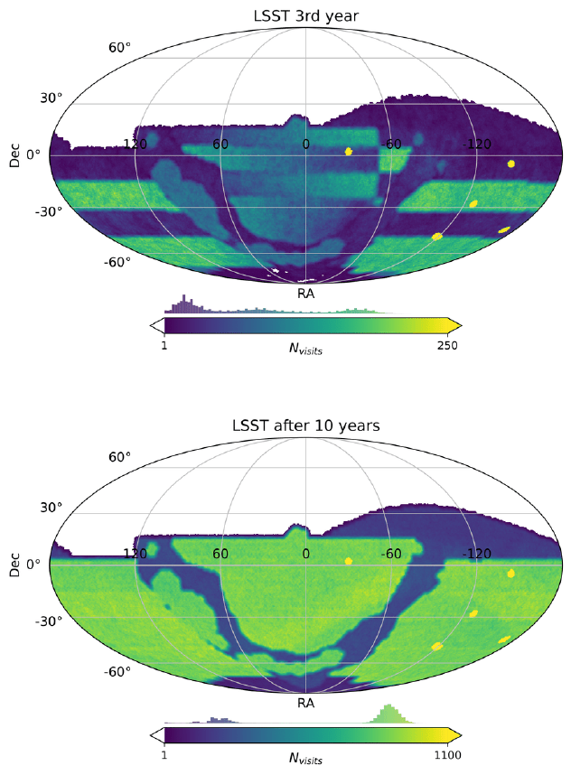
LSST simulations
- 10 year simulation from Uchuu-UniverseMachine (Behroozi et al. 2019)
- Cadence and instrument properties from the observing strategy simulation v3.3
Rosselli et al. 2025
LSST simulations
-
SN host redshift efficiency (C. Ravoux, P. Gris, D. Rosselli, J. Bautista):
- Use of DC2 LSST simulation with galaxy properties
- Footprint and efficiency for different spectroscopic survey
- Considering SNe variety contamination
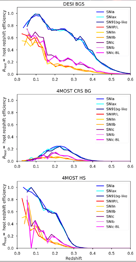
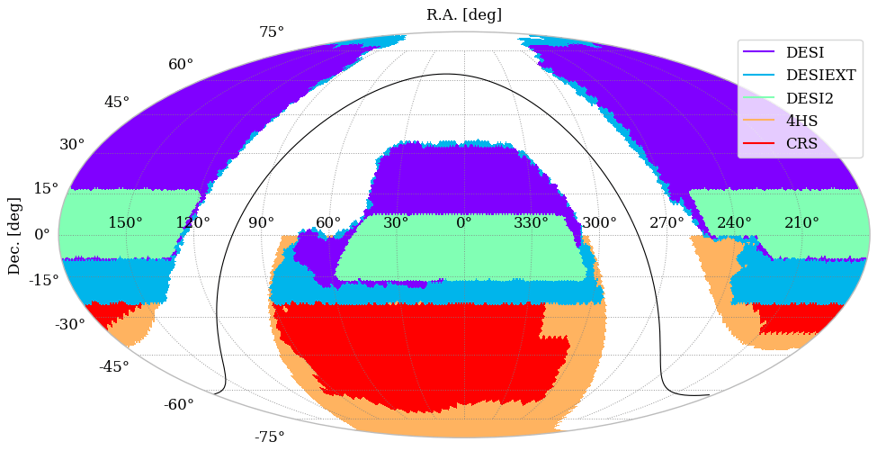
Rosselli et al. 2025
LSST simulations
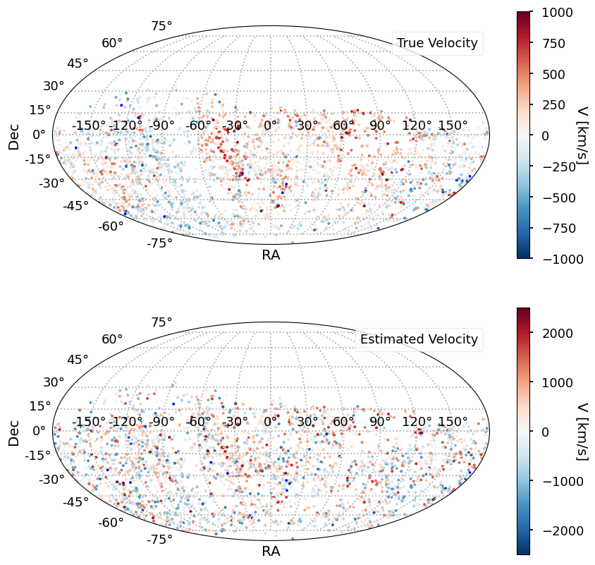
- 33,000 SNe Ia with spectro-z at z < 0.16 (among 1M for the full sample)
- Photo-typing with SuperNNovae (Moller et al. 2019) gives 0.02% contamination from peculiar SN
Rosselli et al. 2025
LSST results
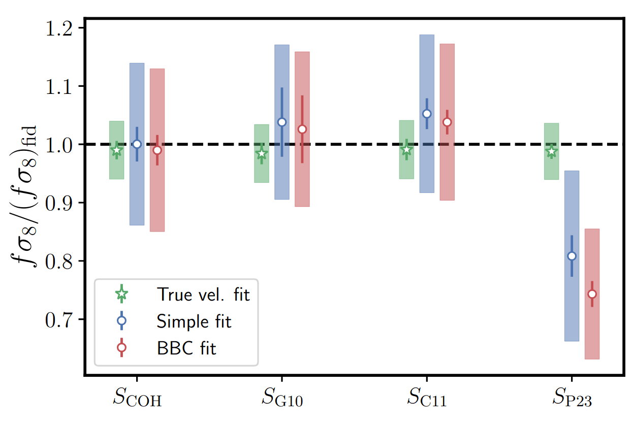
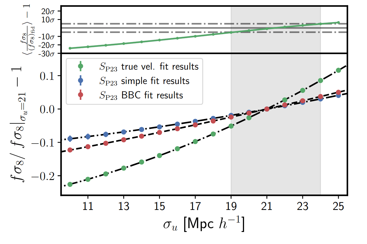
- Dedicated study to test BBC framework and check the impact of intrinsic scatter model and nuisance parameter ( = dispersion of velocity position)
Carreres et al. 2025
LSST results
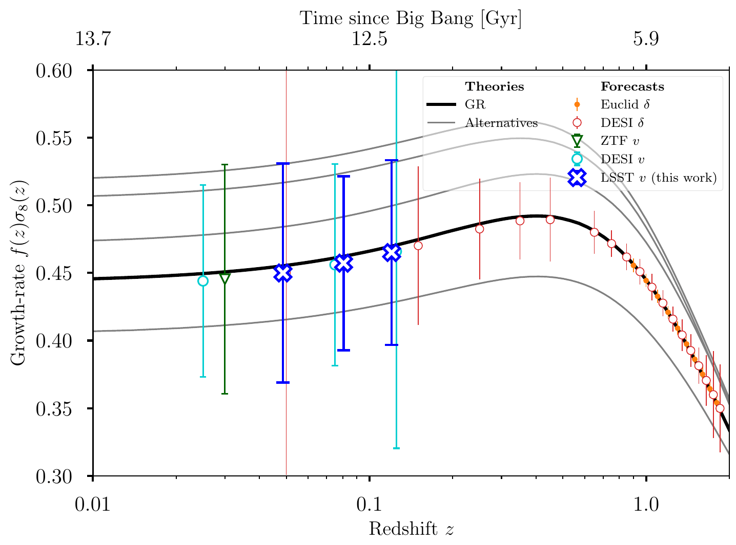
- Unbiased fσ8 measurement with full Hubble diagram fit over 3 redshift points
- How can we do better ? Combine with density field
Rosselli et al. 2025