Growth rate from SNIa peculiar velocity and galaxy density field
Corentin Ravoux
Group presentation - 04/12/25

ACCEL² simulation
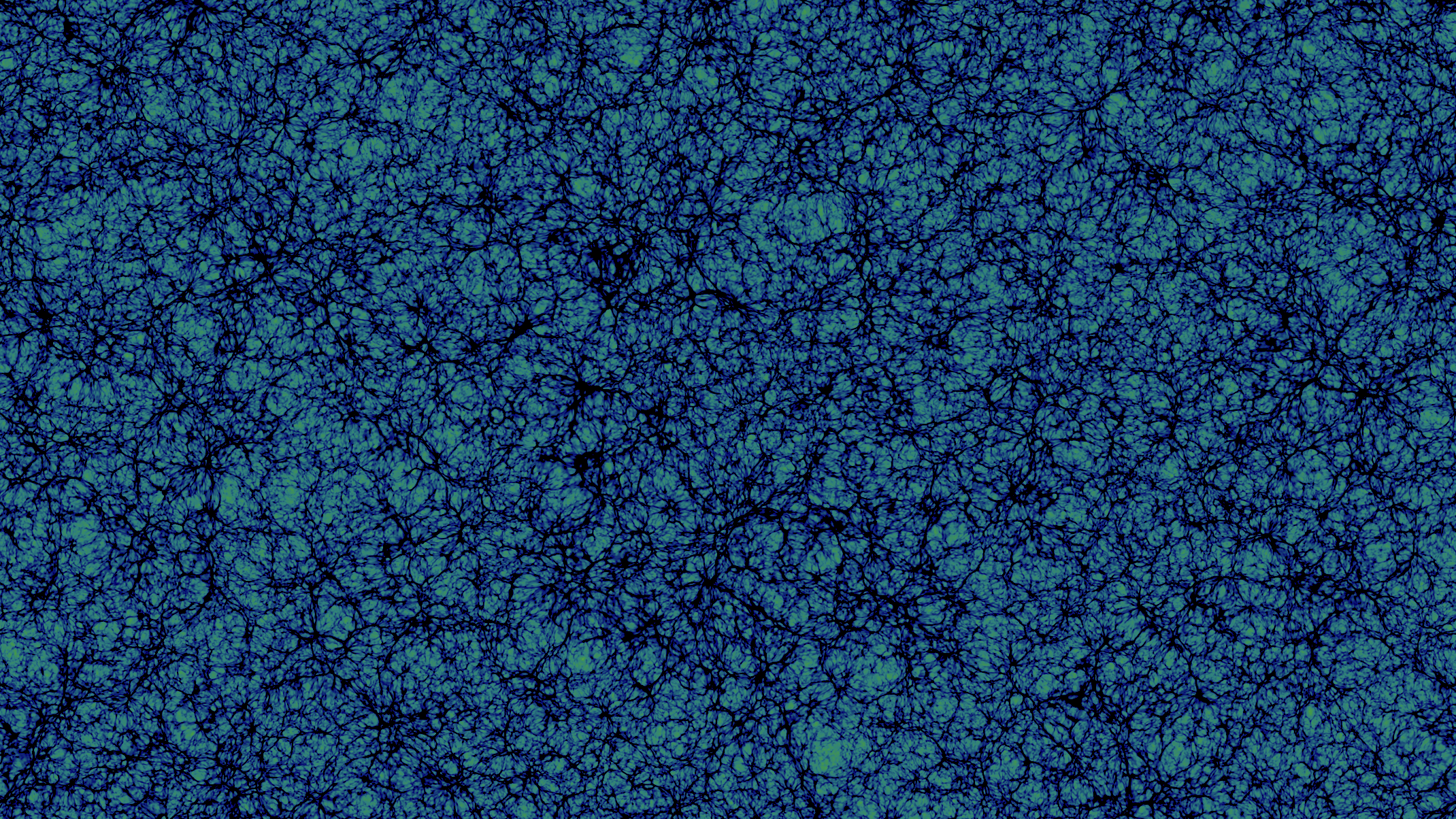
Dark Energy
- What is the nature of dark energy ?
- Cosmological constant model (Λ) not very satisfying
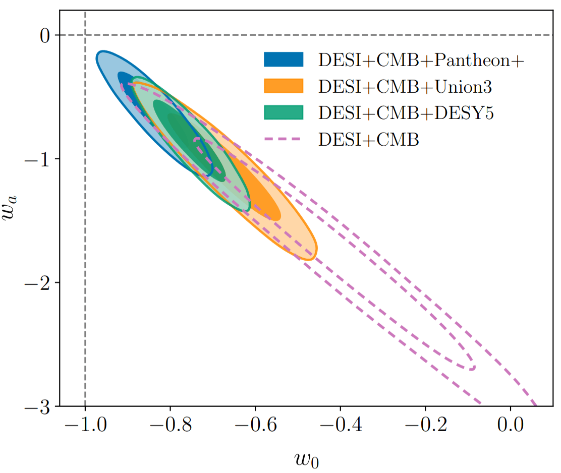
Recent DESI DR2 BAO + CMB + SNIa results: stronger hints for varying dark energy
DESI DR2 BAO 2025
Corentin Ravoux Group presentation - Dec. 2025
Dark Energy
- What is the nature of dark energy ?
- Cosmological constant model (Λ) not very satisfying
-
Other models :
- Fifth force, additional field ?
- Modified gravity theories ?
- Our current objective: Probing large-scale structure formation to constrain dark energy/modified gravity.
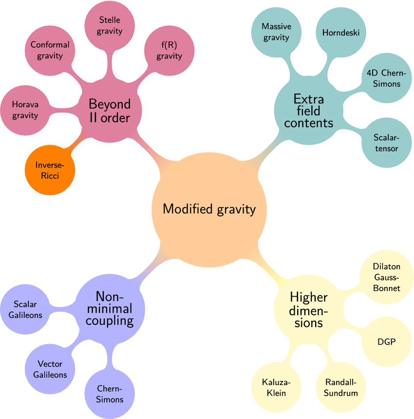
Shankaranarayanan et al. 2022
Corentin Ravoux Group presentation - Dec. 2025
Cosmic web
- Matter perturbations in the primordial Universe grew to form the cosmic web
- Static description: matter density contrast (δ) follows a linear power spectrum at large-scales
- Dynamic description: Cosmic web peculiar velocities ( ) caused by gravitation
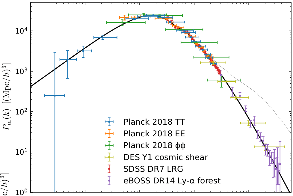

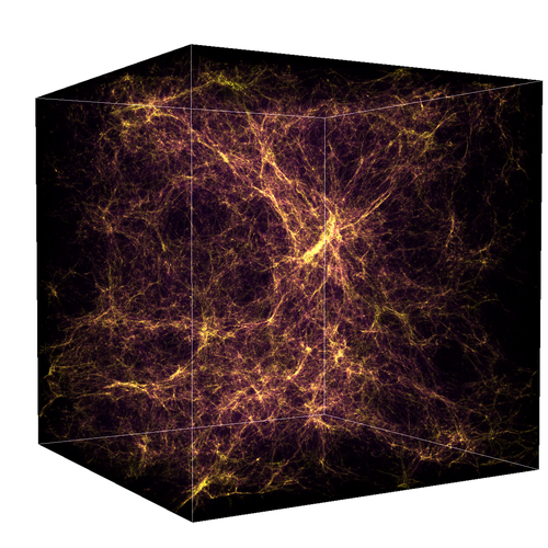
Walther et al. 2021
Chabanier et al. 2019
Corentin Ravoux Group presentation - Dec. 2025
fσ8 parameter
- Linear perturbation theory:
Cosmic web velocities
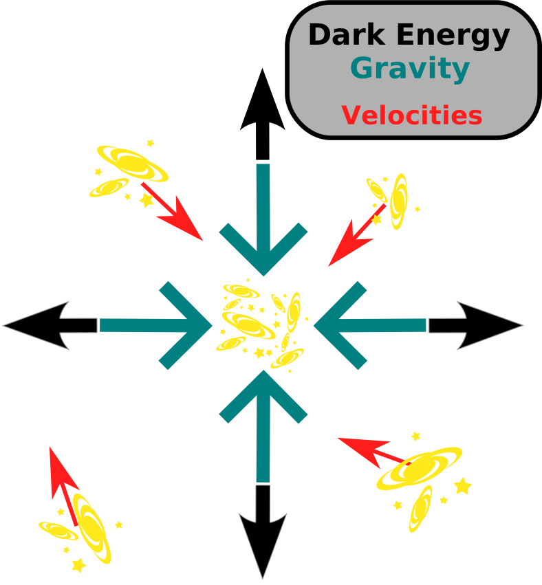
Normalized matter overdensity
Corentin Ravoux Group presentation - Dec. 2025
fσ8 parameter
- Linear perturbation theory:
Cosmic web velocities
Normalized matter overdensity
Logarithmic growth rate of linear perturbations
8 Mpc/h
Amplitude of the matter perturbations in spheres of 8 Mpc/h comoving radius (matter power spectrum amplitude)
in GR
Corentin Ravoux Group presentation - Dec. 2025
Measuring fσ8
Peculiar velocities (PV)
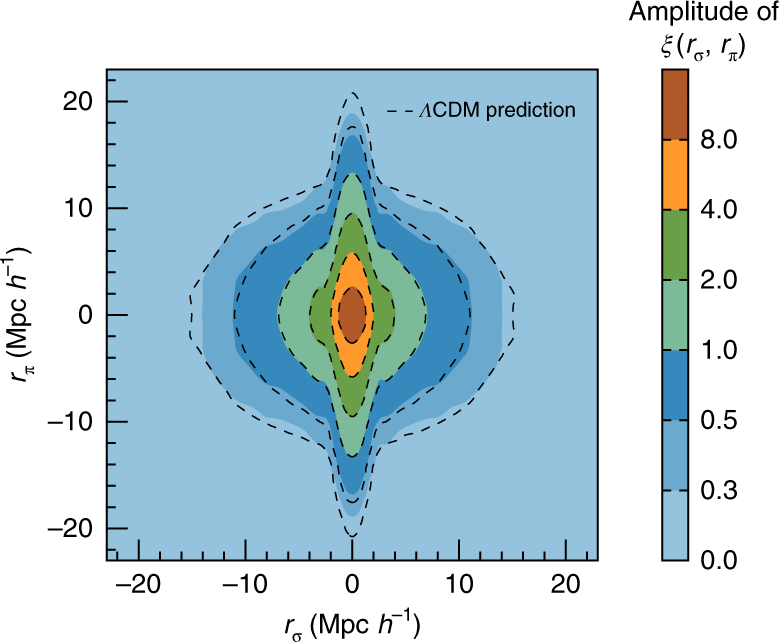
Redshift Space Distortions (RSD)
- Direct estimation of velocities
- Need an estimate of redshift ( ) and distance (decoupling from )
- Compute statistics from PV
- Impact of PV on measurements
- Example: galaxy auto-correlation, void cross-correlation, ...
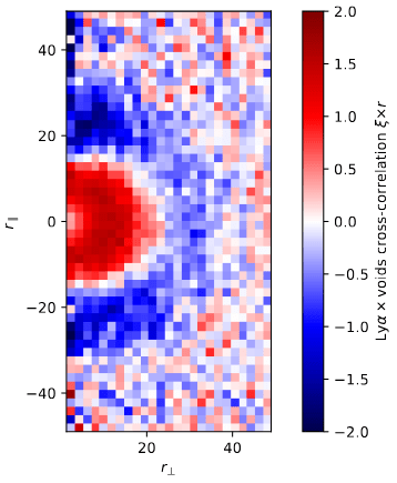
Ravoux et al. 2022
He et al. 2018
Corentin Ravoux Group presentation - Dec. 2025
fσ8 constraints
- Constrain modified gravity models
- RSD very effective for high redshift
- PV for low redshift
- Improvement with method combination
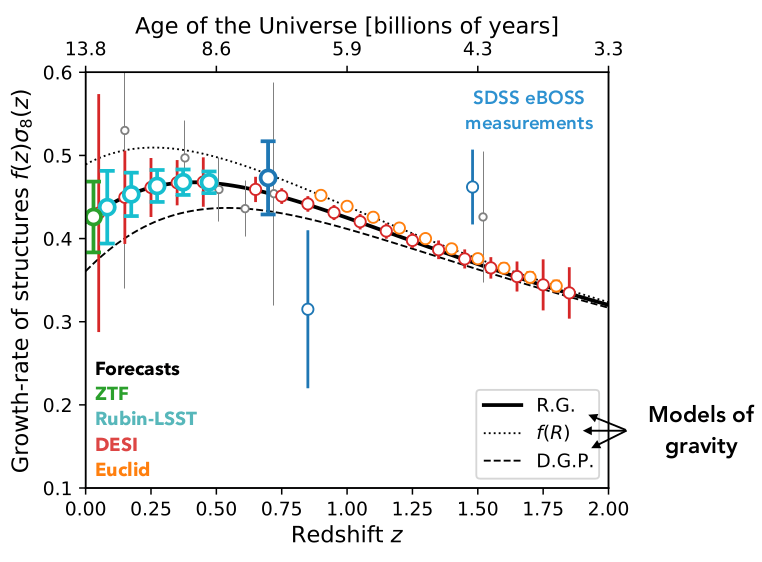
from Julian Bautista
Corentin Ravoux Group presentation - Dec. 2025
fσ8 measurement with peculiar velocities
ACCEL² simulation
ACCEL² simulation
Corentin Ravoux Group presentation - Dec. 2025
Hubble diagram
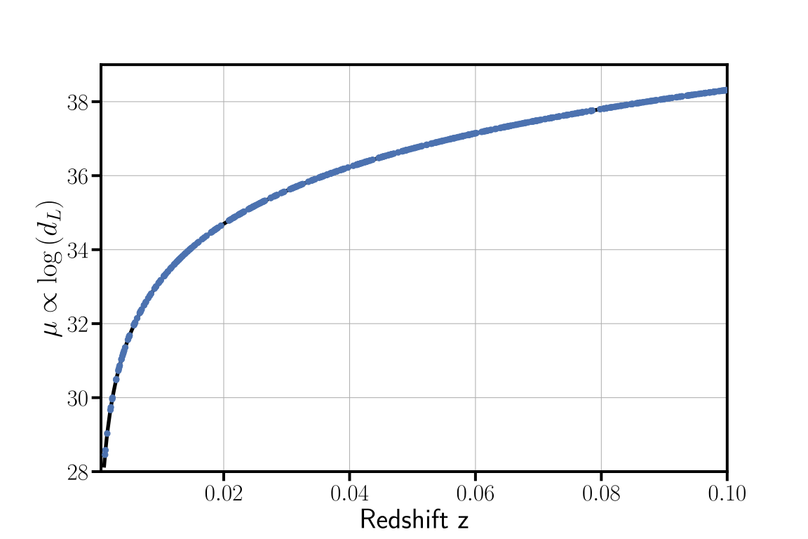
Perfect standard candle in an expanding Universe
from Bastien Carreres
Standard candle = object with fixed luminosity
Corentin Ravoux Group presentation - Dec. 2025
Hubble diagram
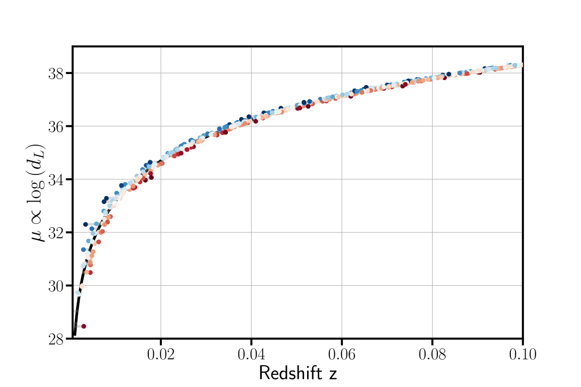
Peculiar velocities
from Bastien Carreres
Perfect standard candle in an expanding Universe
Corentin Ravoux Group presentation - Dec. 2025
Hubble diagram
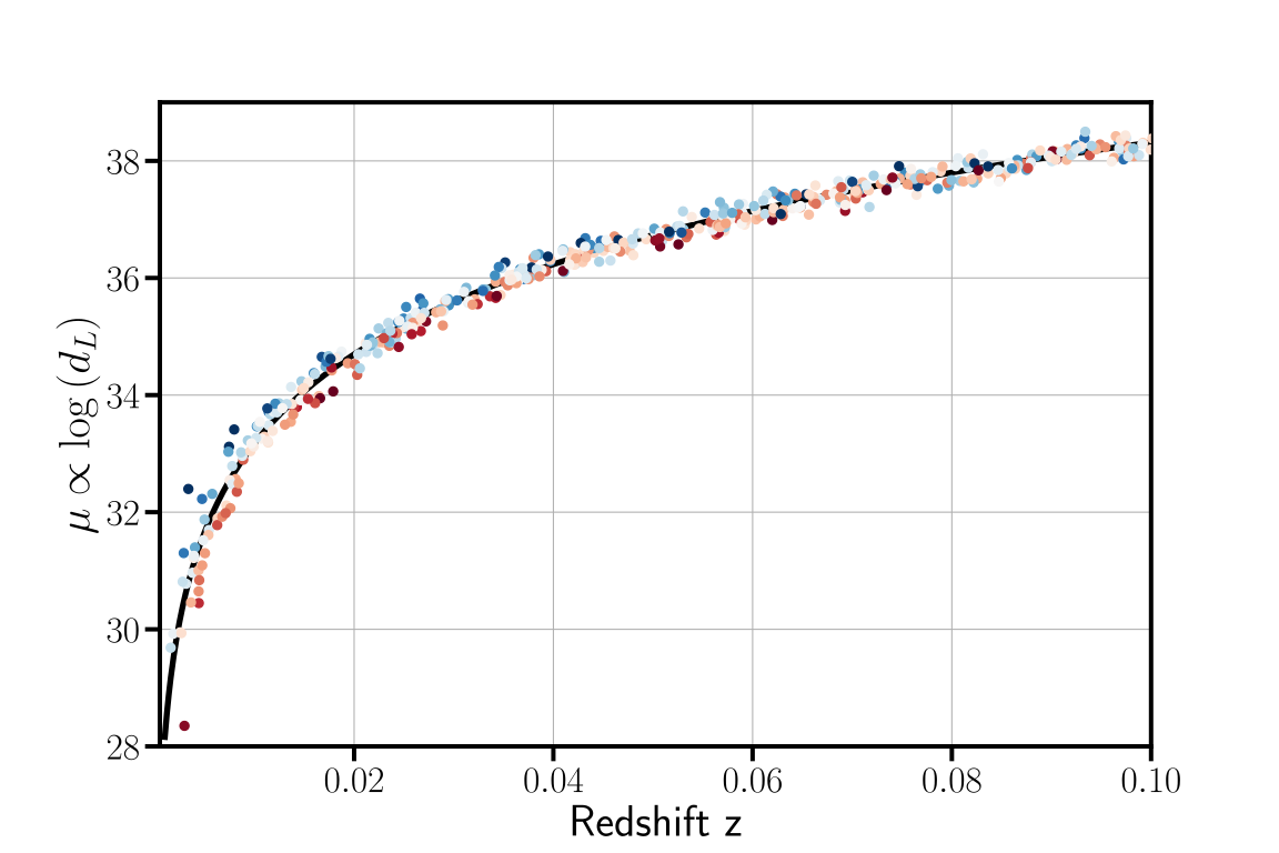
Noise sources (intrinsic scatter, local environment, instruments...)
from Bastien Carreres
Standardizable candle in an expanding Universe
Peculiar velocities
Corentin Ravoux Group presentation - Dec. 2025
Hubble diagram
from Bastien Carreres
Low + High redshifts = dark energy constraints (w, or w0,wa)
Low redshifts + calibration of the candle luminosity = H0 constraints
Hubble residuals = fσ8 constraints
Corentin Ravoux Group presentation - Dec. 2025
"Not-so" standard candles
Tully-Fisher relation
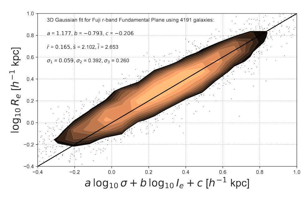
Fundamental plane relation
- Spiral galaxies (Late-type)
- Absolute magnitude (M) / rotational velocity (W)
- Elliptical galaxies (Early-type)
- Effective radius (Re) / surface brightness (Ie) / stellar velocity dispersion (σ)
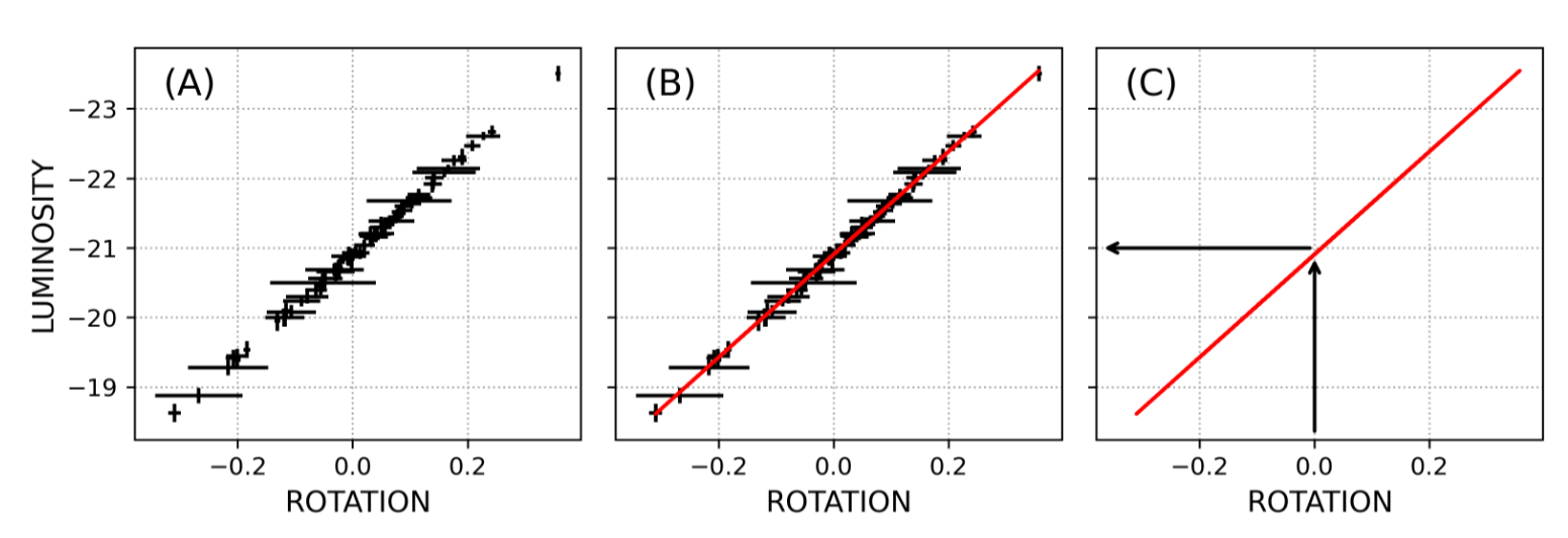
Said et al. 2024
Said 2023
Corentin Ravoux Group presentation - Dec. 2025
Type Ia supernovae
- Distance modulus:
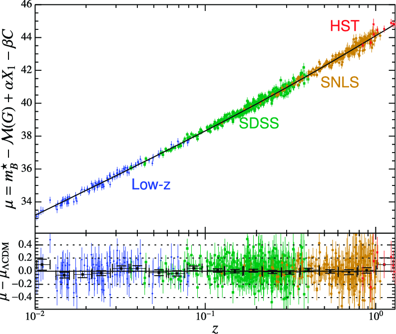
Betoule et al. 2014
- SNe Ia standardization = Tripp relation
Light-curve stretch
SN color
Parameters common for all SN Ia
"Redder is fainter"
"Luminous fade slowly"
- SNe Ia: Thermonuclear explosion a white dwarf reaching Chandrasekhar mass
Corentin Ravoux Group presentation - Dec. 2025
Type Ia supernovae
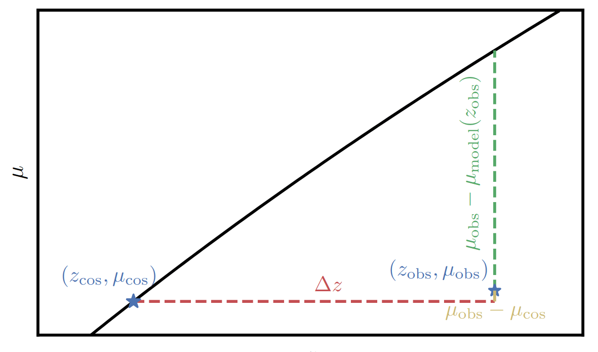
- Hubble residuals:
- Velocity estimator:
Carreres et al. 2023
Corentin Ravoux Group presentation - Dec. 2025
Likelihood-based field-level inference
ACCEL² simulation
ACCEL² simulation
Carreres et al. 2023
Ravoux et al. 2025
Corentin Ravoux Group presentation - Dec. 2025
Likelihood-based field-level estimator
Velocity from SNe Ia
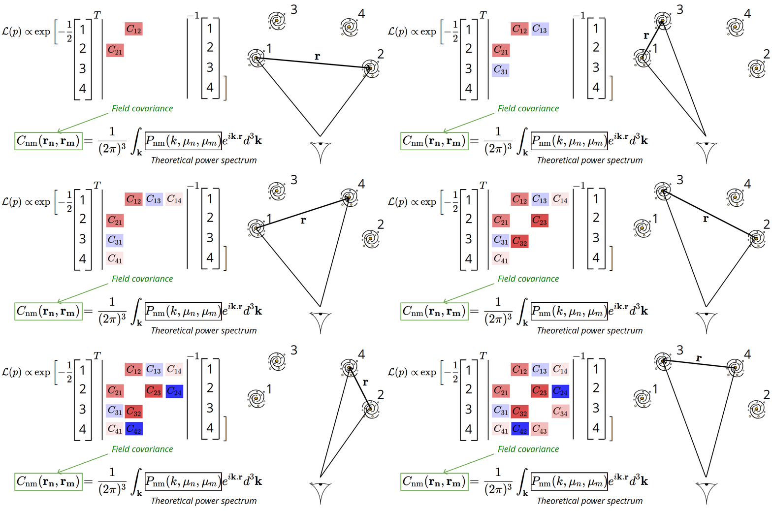
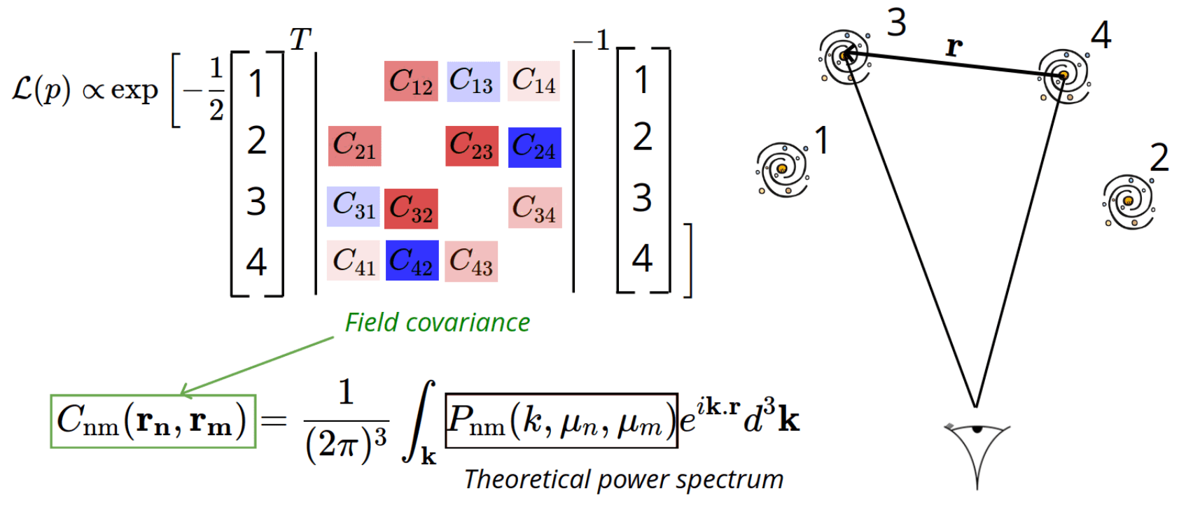
Field covariance matrix computed from theory and coordinates
Parameters
Velocity example:
- Standard inference: compute 2-point correlation functions and fit
- Field-level inference: Maximizing or sampling a likelihood computed from all coordinates of the data
- p = fitted parameters: simultaneously cosmology (fσ8) and field parameters (e.g., Hubble diagram parameters α, β, M0 for SN)
Corentin Ravoux Group presentation - Dec. 2025
Computing the field covariance
Corentin Ravoux Group presentation - Dec. 2025
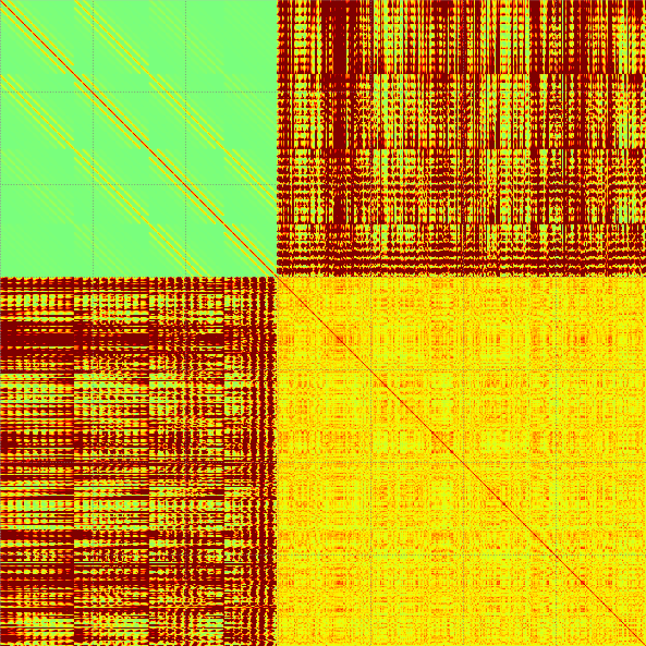
Combining densities (RSD) and peculiar velocities
Velocities
Density field from galaxy surveys
Full field covariance matrix
Corentin Ravoux Group presentation - Dec. 2025
General covariance calculation
- Objective: Improve/Extend the likelihood-based modeling
- General form of field power spectrum
- Algorithmically-oriented calculations (Hankel transforms)
- Wide-angle effect accounted in the integration
gg, gv, vv
Parameters to fit
Terms to integrate analytically
Power spectra terms to integrate numerically
Corentin Ravoux Group presentation - Dec. 2025
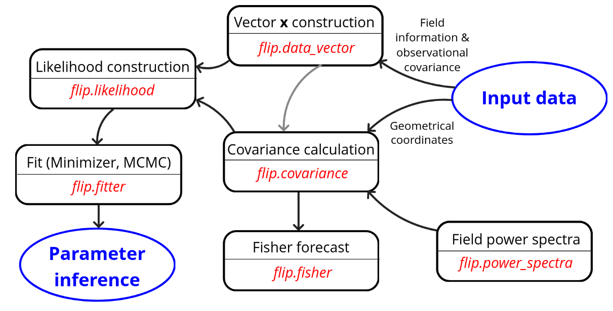
flip Field Level Inference Package
- python package for likelihood-based field-level inference:
https://github.com/corentinravoux/flip
- Fast generation of field covariance
- Symbolic code generation for covariance model
- MCMC and Minuit to fit fσ8
- General expression for vectors (SNIa, density, log distance, TF, FP...)
- Survey geometry-dependent Fisher forecast

Contributors: Bastien Carreres, Damiano Rosselli and Alex G. Kim
Flip article: arxiv:2501.16852
Corentin Ravoux Group presentation - Dec. 2025
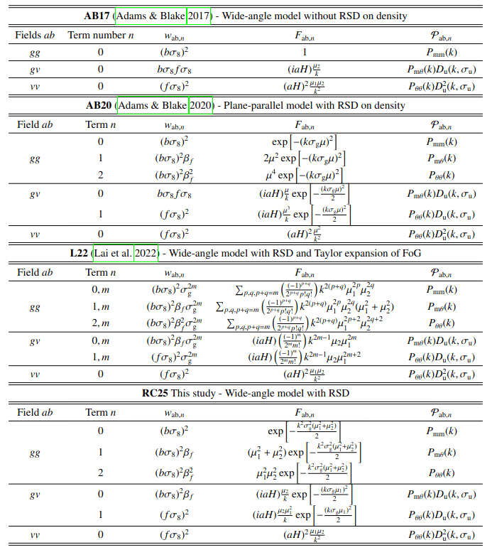
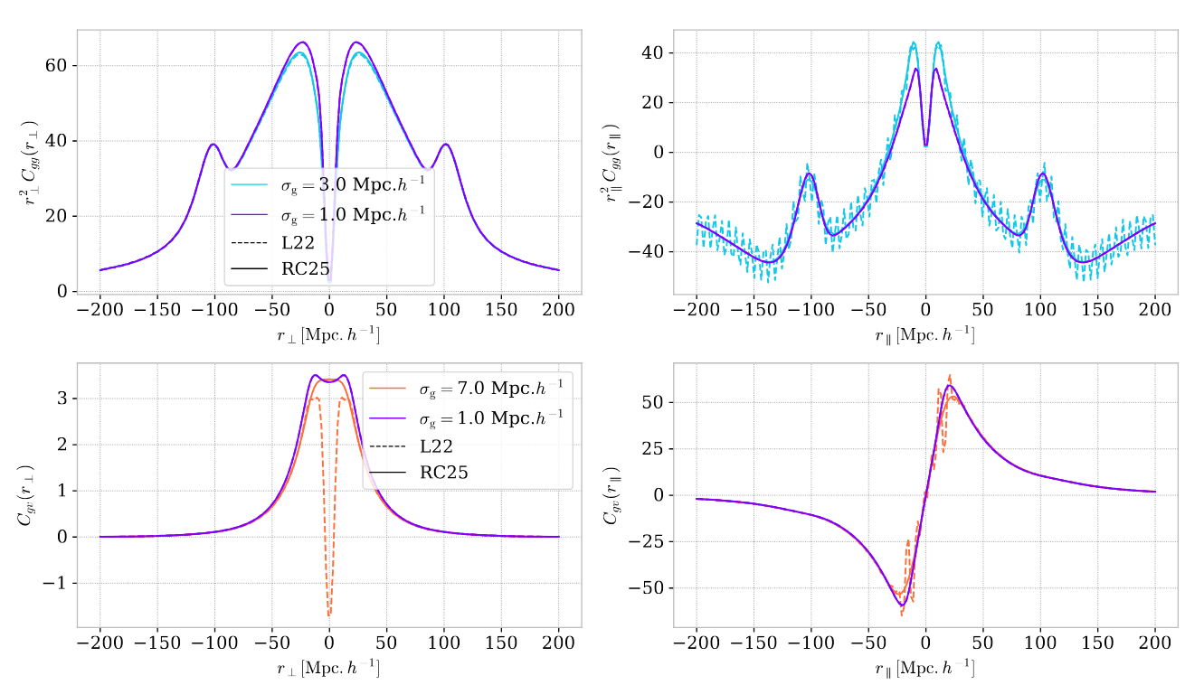
Field covariance models
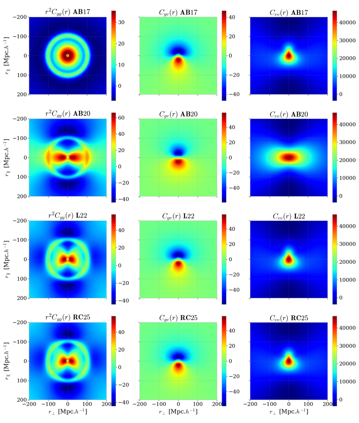
- Model comparison on a regular coordinate grid (Adams & Blake 2017, Adams & Blake 2020, Lai et al. 2022)
- New wide-angle model developed (RC25): improved stability in integration and for wider fitting parameter ranges
Ravoux et al. 2025
Corentin Ravoux Group presentation - Dec. 2025
Combining DESI galaxy density and ZTF SNIa velocities on simulation
ACCEL² simulation
ACCEL² simulation
Ravoux et al. in prep
Corentin Ravoux Group presentation - Dec. 2025
ACCEL² simulation
Zwicky Transient Facility (ZTF)
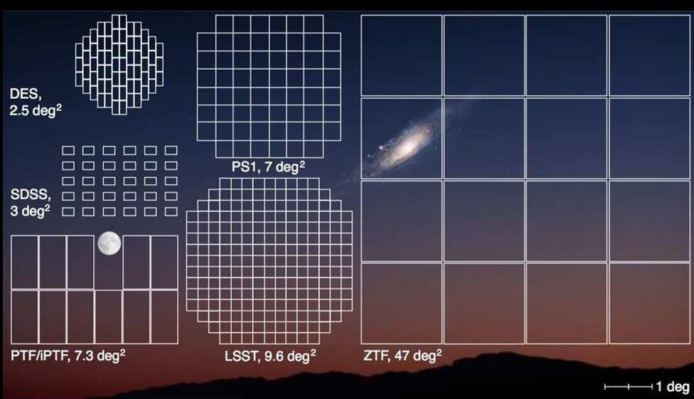
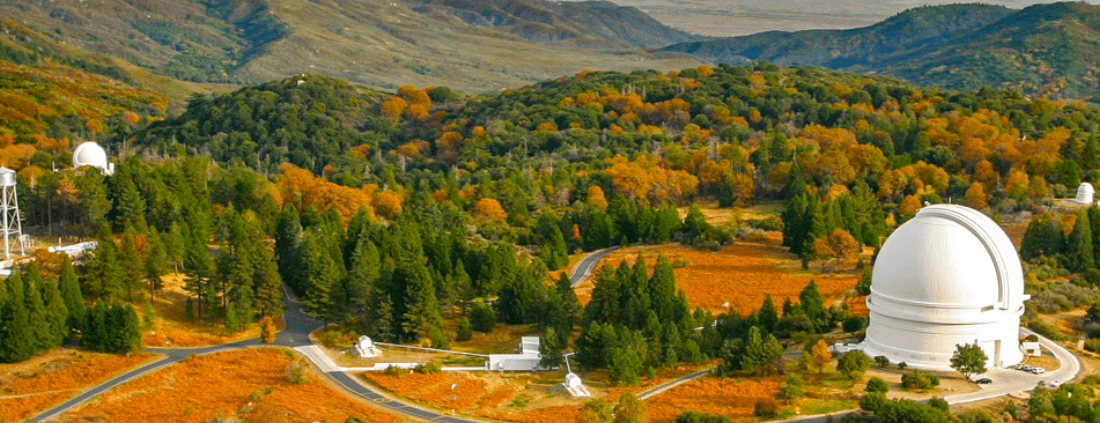
- ZTF = high-cadence photometric telescop in the Palomar observatory
- Very large field of view (47 deg²)
- Observing 3/4 of the sky every nights with 3 filters (g, r, i)
- Transient sky: Supernovae, gamma ray burst, tidal distruptive events, comets, asteroids
-
Dedicated spectroscopic telescope measuring transient spectra (SEDmachine)
Corentin Ravoux Group presentation - Dec. 2025
SN Ia simulation and analysis

SN Ia simulator
Survey parameters
SN Ia model
N-body host simulation
Realistic SN Ia light curves
Quality cuts
(Detection, spec-z selection, light curve quality...)
Light curve fit (SALT2)
Velocity estimation and simultaneous fit of fσ8 and velocity parameters
Simulation
Analysis
Corentin Ravoux Group presentation - Dec. 2025
snsim
https://github.com/bastiencarreres/snsim
- Survey parameters: Cadence (ZTF, LSST), CCD gain, zero point, sky noise
- SN Ia model: Rate, SED, color, stretch, intrinsic scattering distributions, light-curve parameters
- Host catalog: Use velocities and associated clustering from N-body simulation
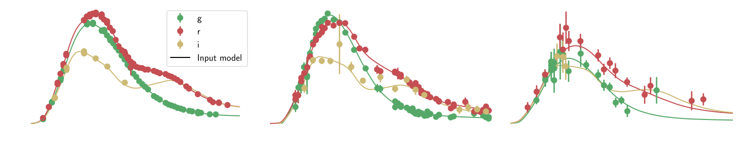
Flux
Phase
Phase
Phase
Carreres et al. 2023
Main contributors: Bastien Carreres, Damiano Rosselli
Corentin Ravoux Group presentation - Dec. 2025
DESI
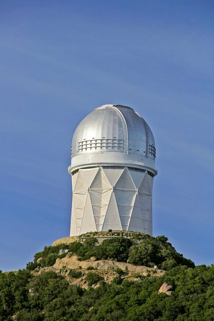
- 4m multi-object spectrograph at Kitt Peak Observatory
DESI collaboration 2022
Corentin Ravoux Group presentation - Dec. 2025
DESI
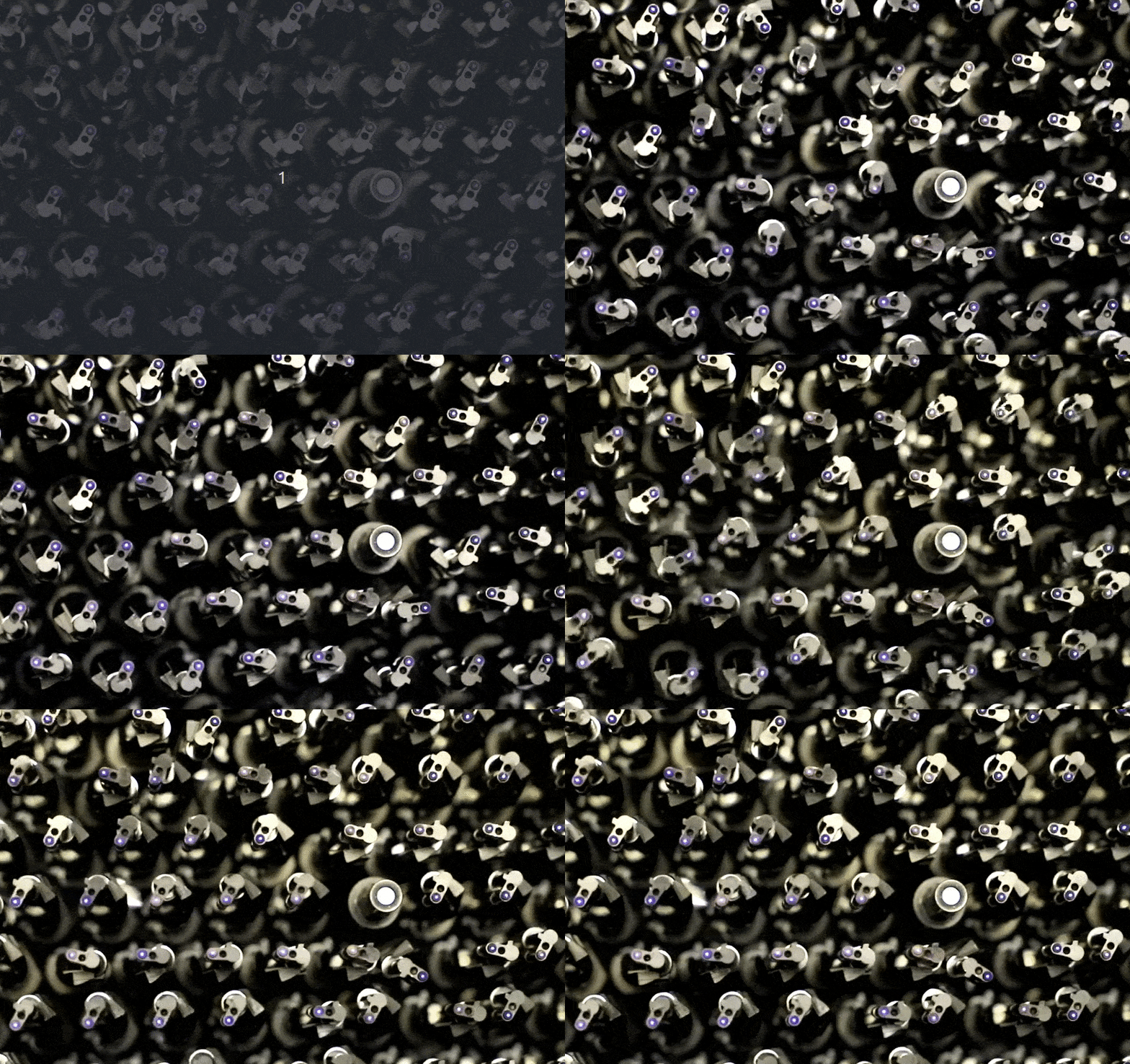
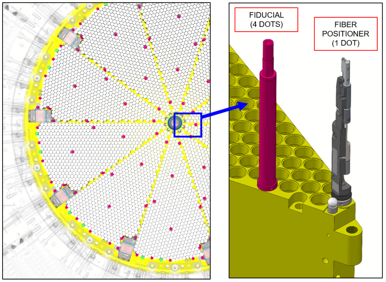
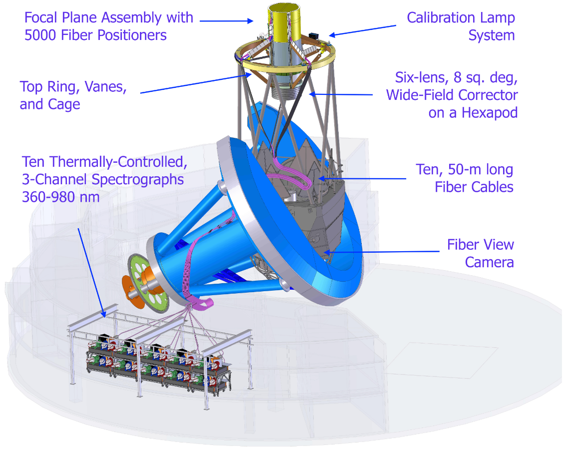
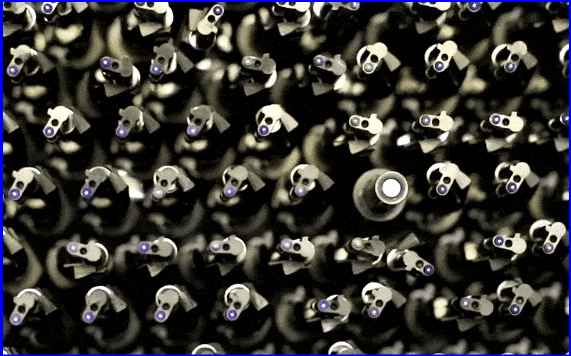
- 5 μm positioning in few sec. for 5000 targets
- All fibers connected to 10 spectrographs
Silber et al. 2022
Corentin Ravoux Group presentation - Dec. 2025
DESI
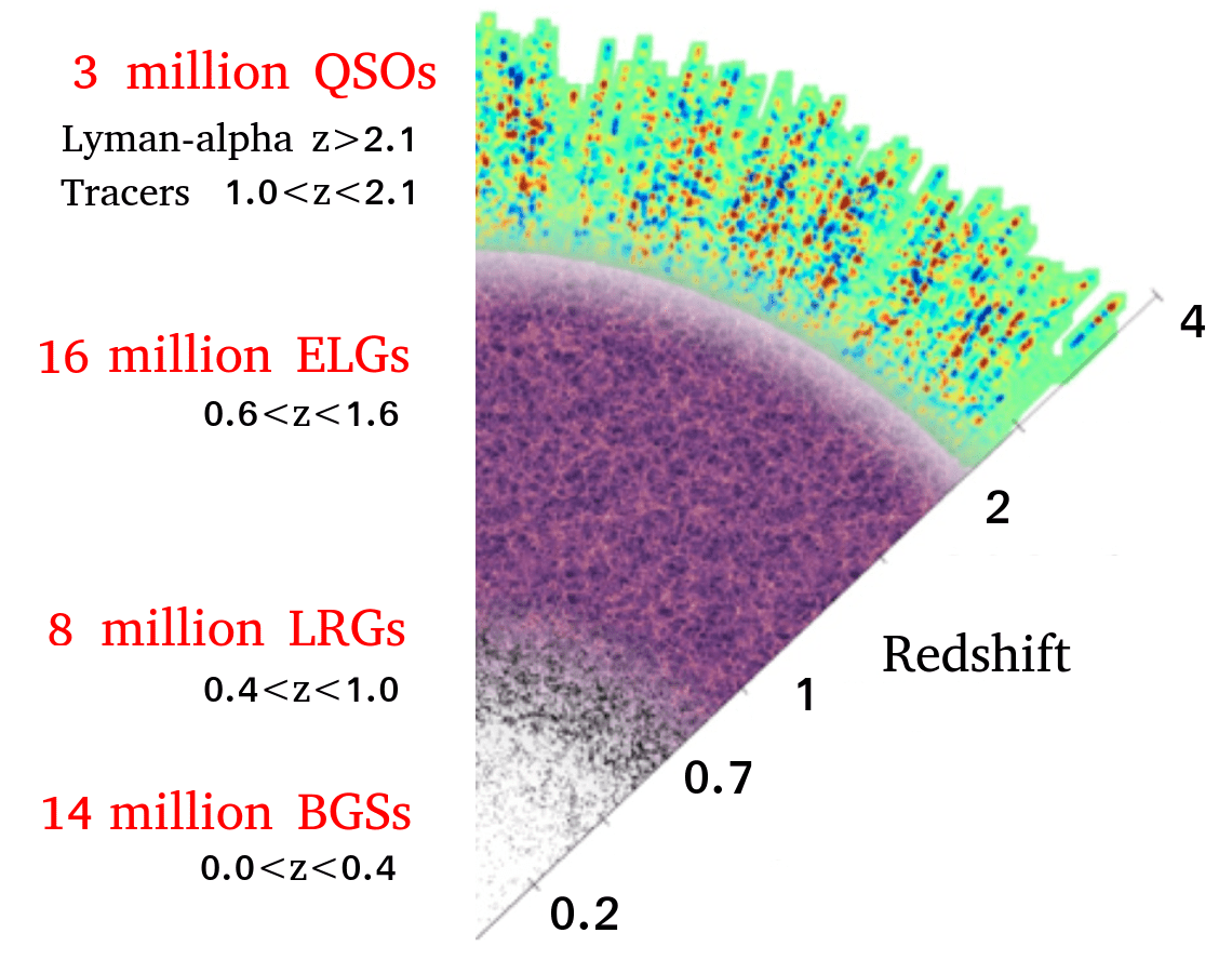
- BGS: Bright Galaxy Survey
- LRG: Luminous Red Galaxy
- ELG: Emission Line Galaxy
-
QSO: Quasar
- z > 2.1: with a Lyman-α forest
- z < 2.1: as tracers
63 million redshifts in 8 years
over 17,000 deg²
Primary science: BAO and RSD measurements
21
12
24
5
Corentin Ravoux Group presentation - Dec. 2025
DESI x ZTF simulation
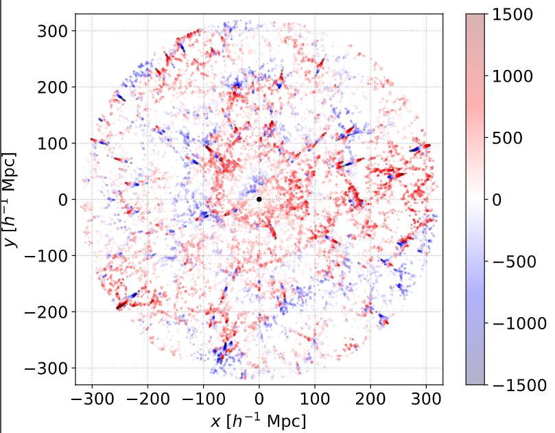
- 27 simulations from AbacusSummit (Maksimova et al. 2019)
- Density: DESI Bright Galaxy Survey (BGS) clustering matching for DR3 (J. Bautista, A. Smith)
- Velocity: ZTF SNIa Y6 simulation performed (following Carreres et al. 2023)
from Julian Bautista
Corentin Ravoux Group presentation - Dec. 2025
Galaxy field
Supernovae velocities
- Runs of SNsim to mimic ZTF SNIa Y6 data set (following Carreres et al. 2023)
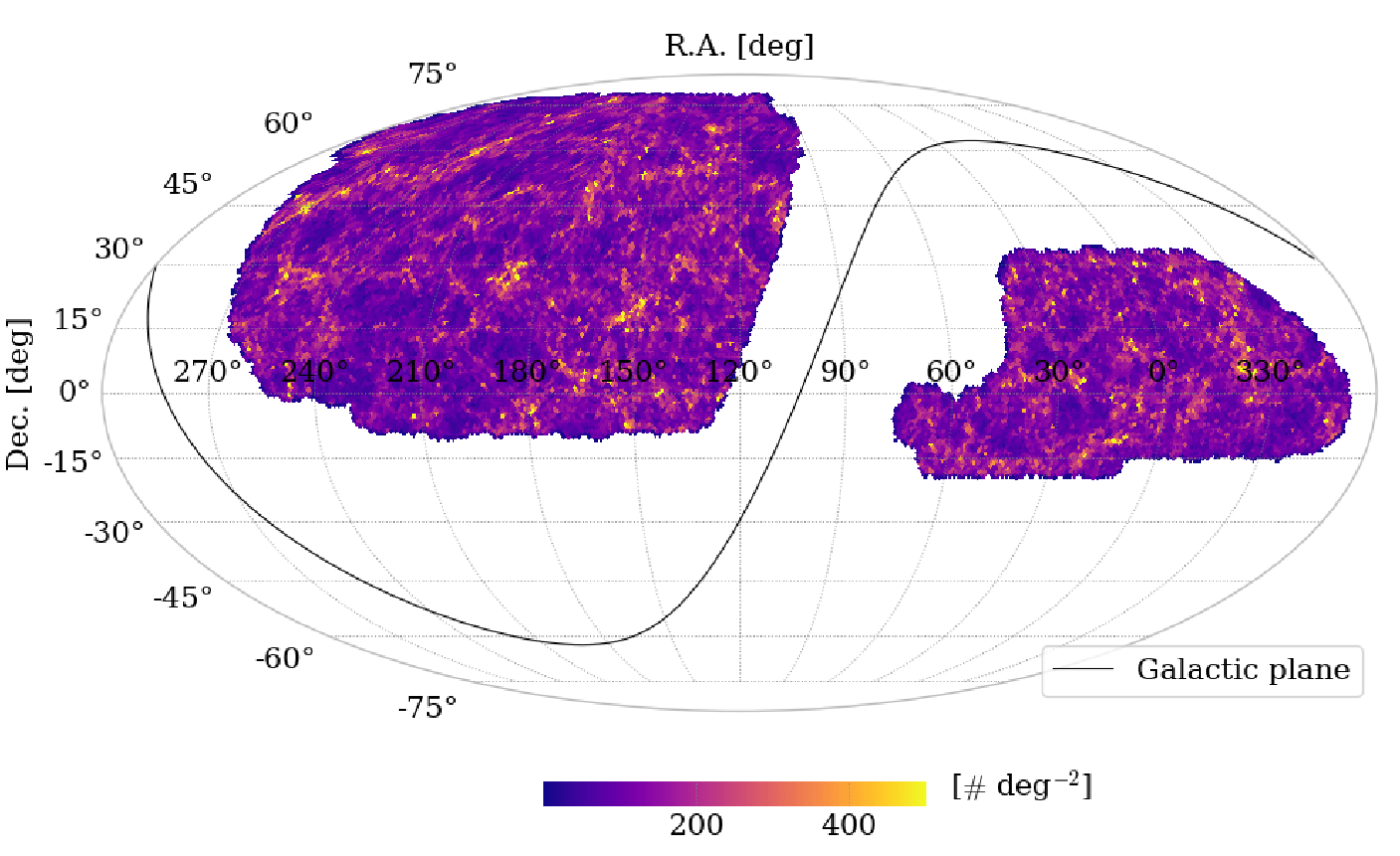
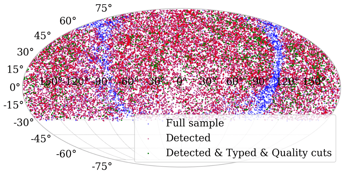
- AbacusSummit mocks matching DESI DR3 (5 years) BGS clustering and footprint
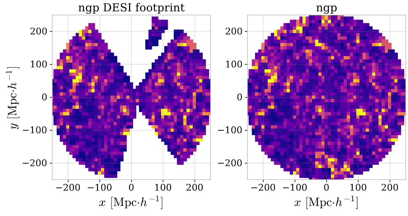
Ravoux et al. in prep.
Corentin Ravoux Group presentation - Dec. 2025
Model for density & velocity fit
- Use of the RC25 wide-angle model implemented in flip:
Corentin Ravoux Group presentation - Dec. 2025
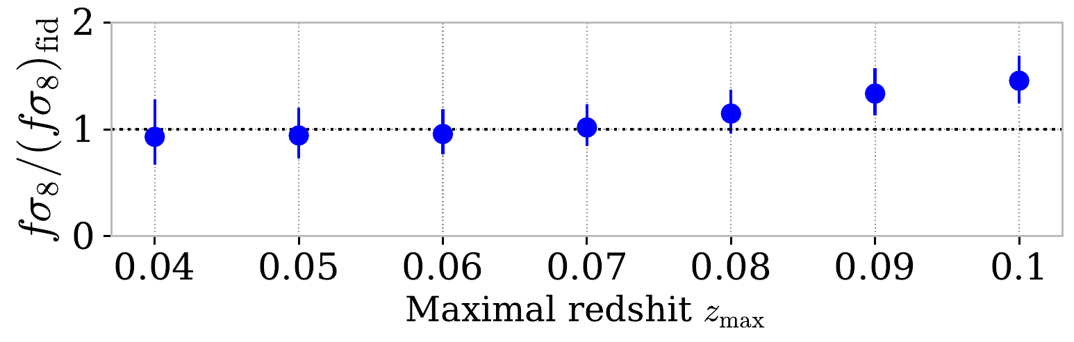
ZTF velocity fit
- Velocity fit including Hubble diagram parameters to reproduce Carreres et al. 2023
- Variation of analysis parameters (max redshift, SNIa density...)
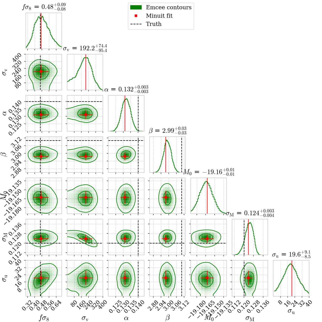
Ravoux et al. in prep.
Corentin Ravoux Group presentation - Dec. 2025
DESI density fit
- Density grid with pypower
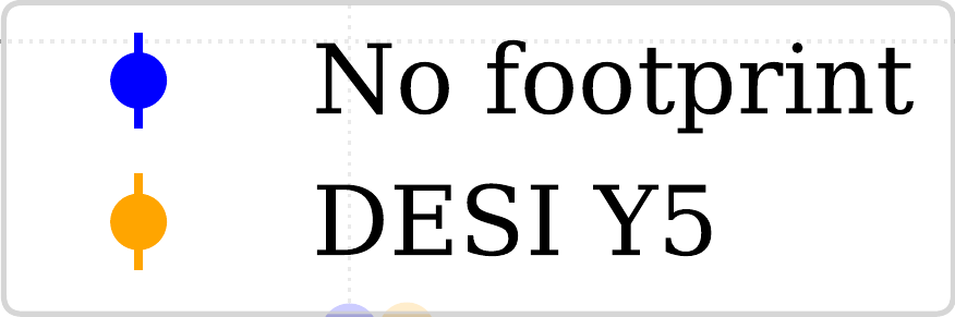
- Test varying all density gridding parameters: grid size, mesh cell size, interpolation scheme (NGC, CIC, TSC, PCS), footprint (DESI DR3 or no cut)
- Mean minuit fit on 27 mocks with average error bar
Ravoux et al. in prep.
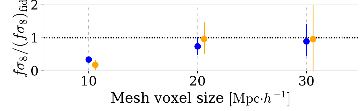
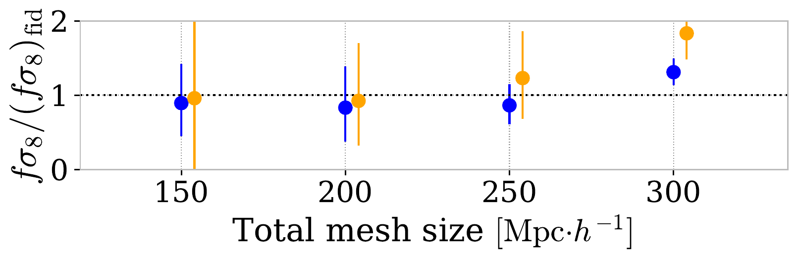
Corentin Ravoux Group presentation - Dec. 2025
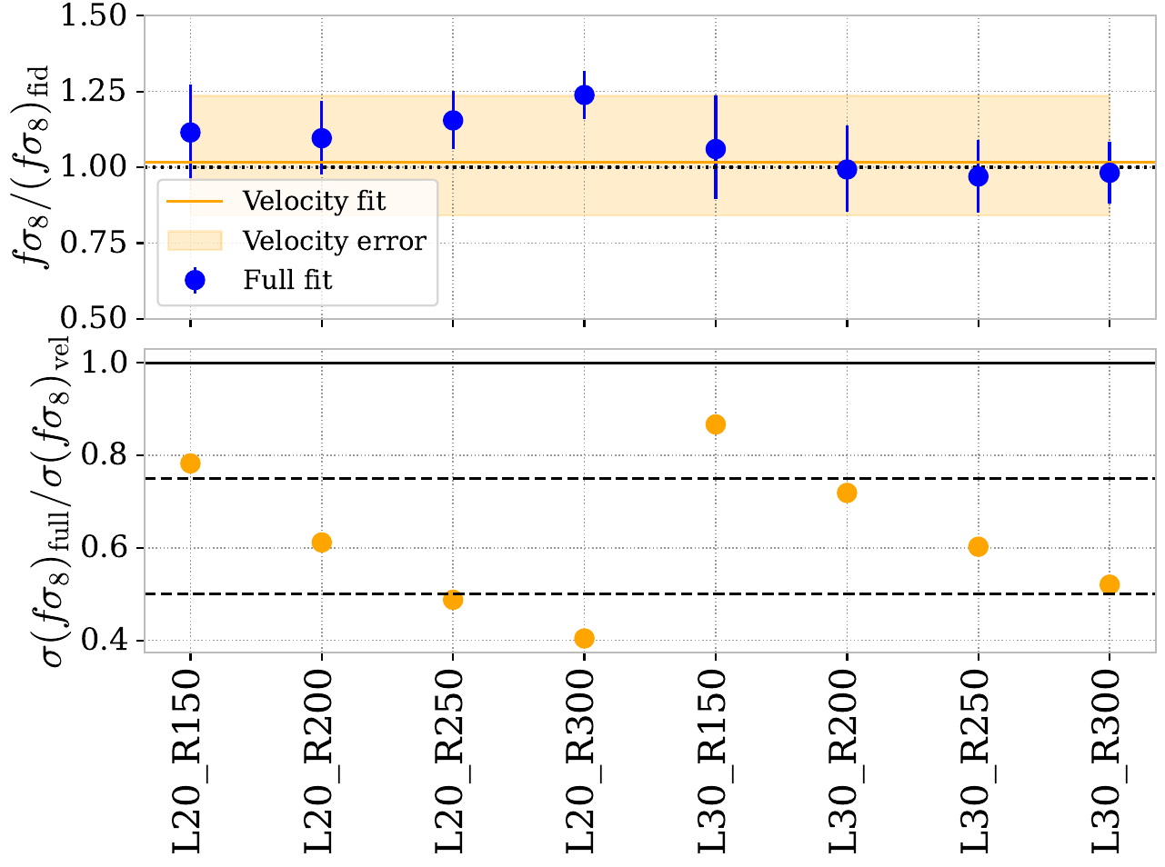
DESI x ZTF joint fit
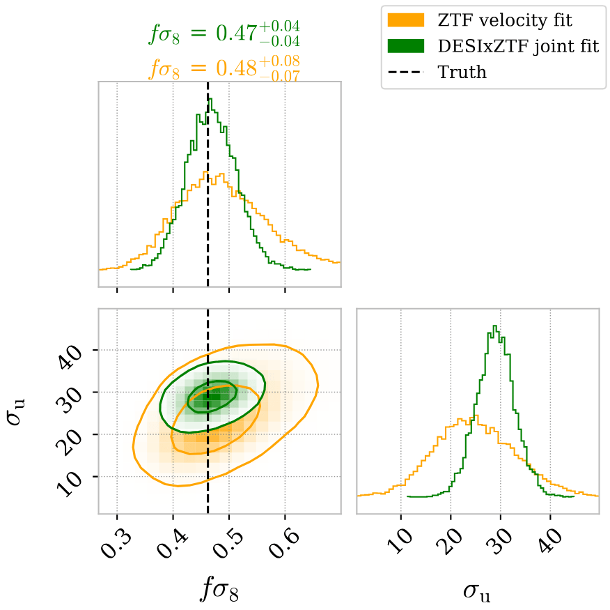
- SNIa velocity fit with Hubble diagram parameters and density field
Adding density improves fs8 constraints up to 60%
Different density configurations
Ravoux et al. in prep.
Corentin Ravoux Group presentation - Dec. 2025
Growth rate on LSST SNIa simulations
ACCEL² simulation
ACCEL² simulation
Carreres et al. 2025
Rosselli et al. 2025
Corentin Ravoux Group presentation - Dec. 2025
Rubin - LSST
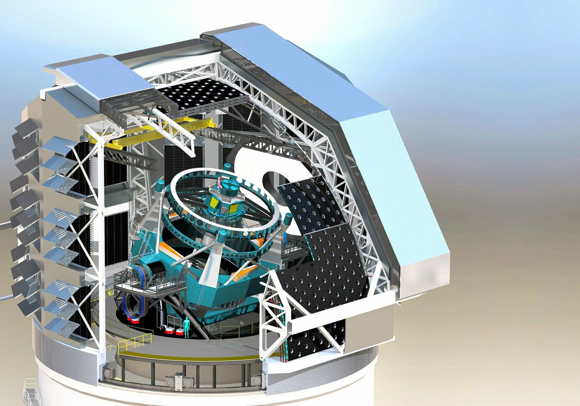
Telescope mount assembly
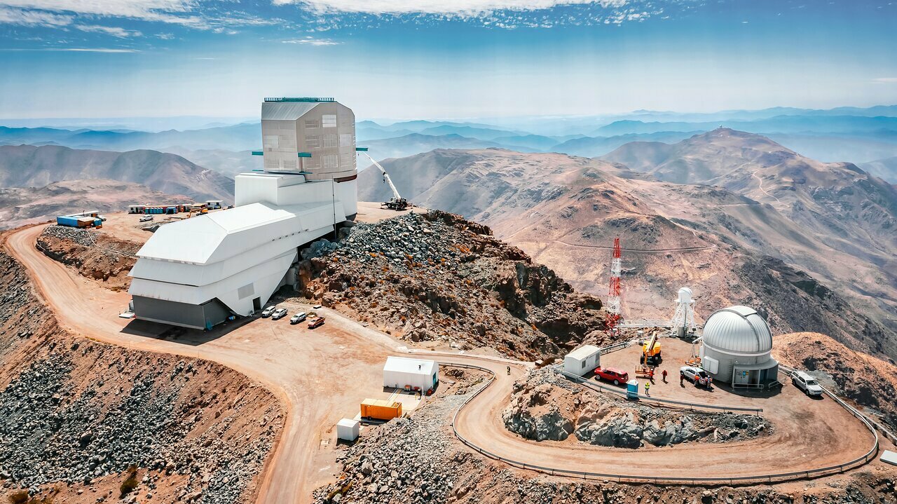
AuxTel: 1.2m atmospheric telescop
Corentin Ravoux Group presentation - Dec. 2025
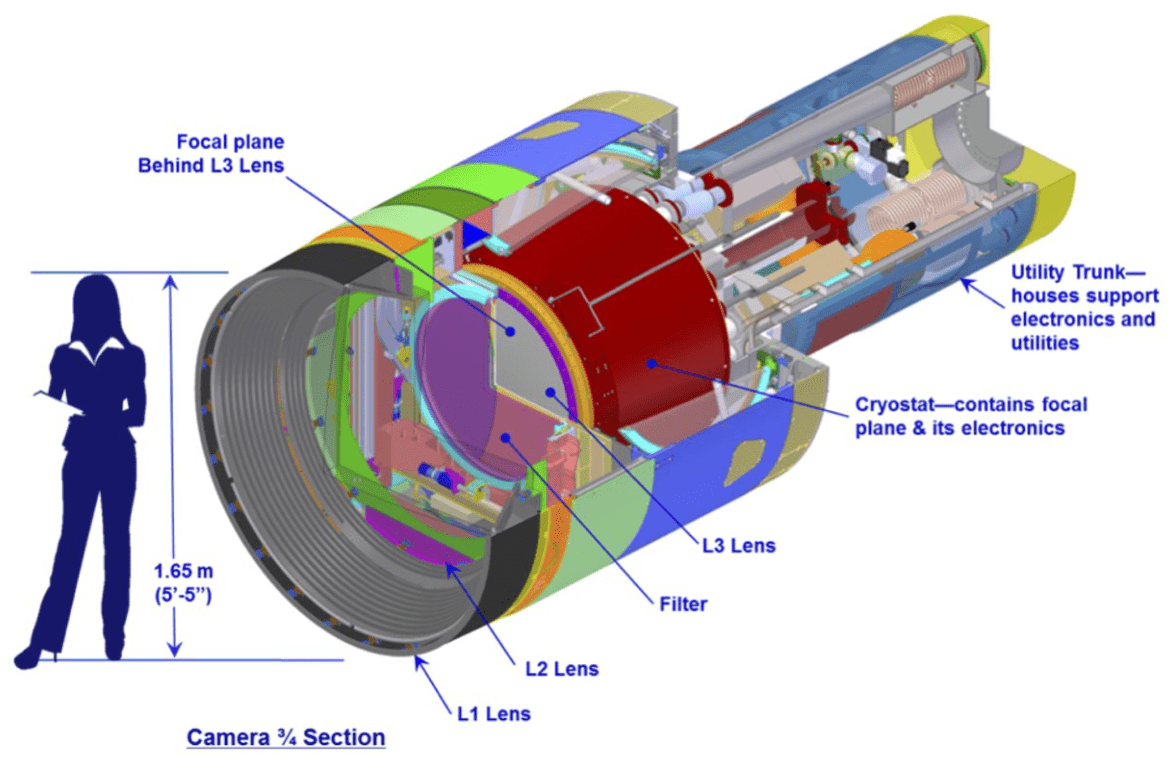
Rubin - LSST: instrument
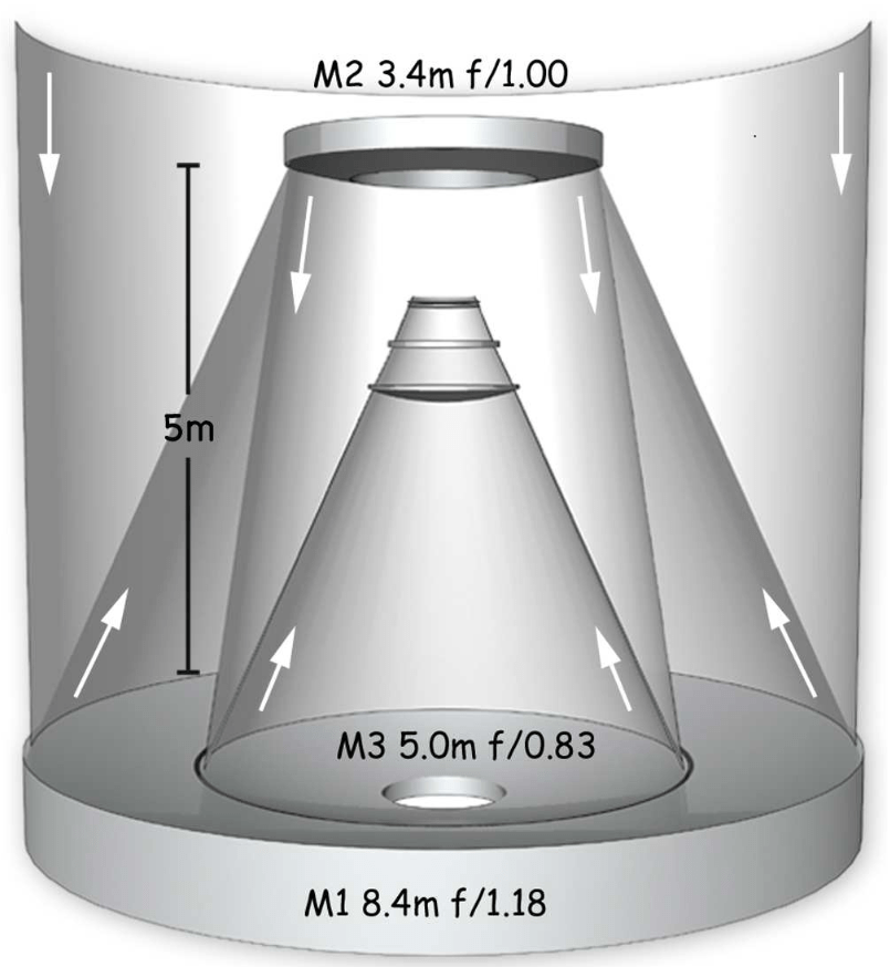
- Largest numerical camera in the world: 3.2 Gpixels with 2s readout time
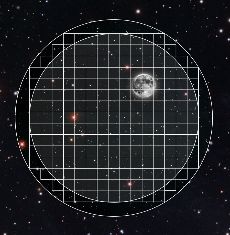
- 8.4 m primary mirror and 9.6 deg² field of view
- 6 filters: (u, g, r, i, z, y)
- 10-year photometric survey of half of the sky (~ 20 000 deg²)
Corentin Ravoux Group presentation - Dec. 2025
LSST simulations
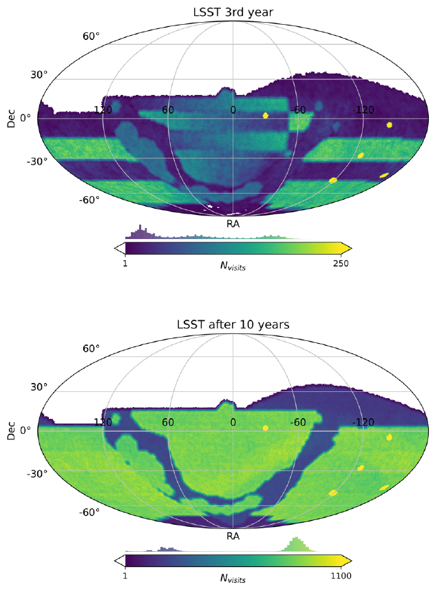
- 10 year simulation from Uchuu-UniverseMachine (Behroozi et al. 2019)
- Cadence and instrument properties from the observing strategy simulation v3.3
Rosselli et al. 2025
Corentin Ravoux Group presentation - Dec. 2025
LSST simulations
-
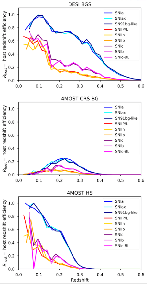
SN host redshift efficiency (C. Ravoux, P. Gris, D. Rosselli, J. Bautista):
- Use of DC2 LSST simulation with galaxy properties
- Footprint and efficiency for different spectroscopic survey
- Considering SNe variety contamination
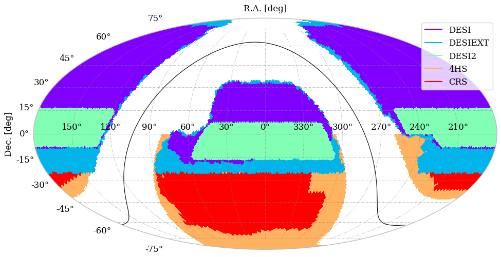
Rosselli et al. 2025
Corentin Ravoux Group presentation - Dec. 2025
LSST simulations
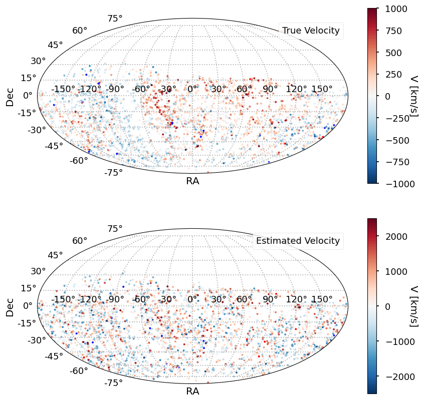
- 33,000 SNe Ia with spectro-z at z < 0.16 (among 1M for the full sample)
- Photo-typing with SuperNNovae (Moller et al. 2019) gives 0.02% contamination from peculiar SN
Rosselli et al. 2025
Corentin Ravoux Group presentation - Dec. 2025
LSST results
- Dedicated study to test BBC framework and check the impact of intrinsic scatter model and nuisance parameter ( = dispersion of velocity position)
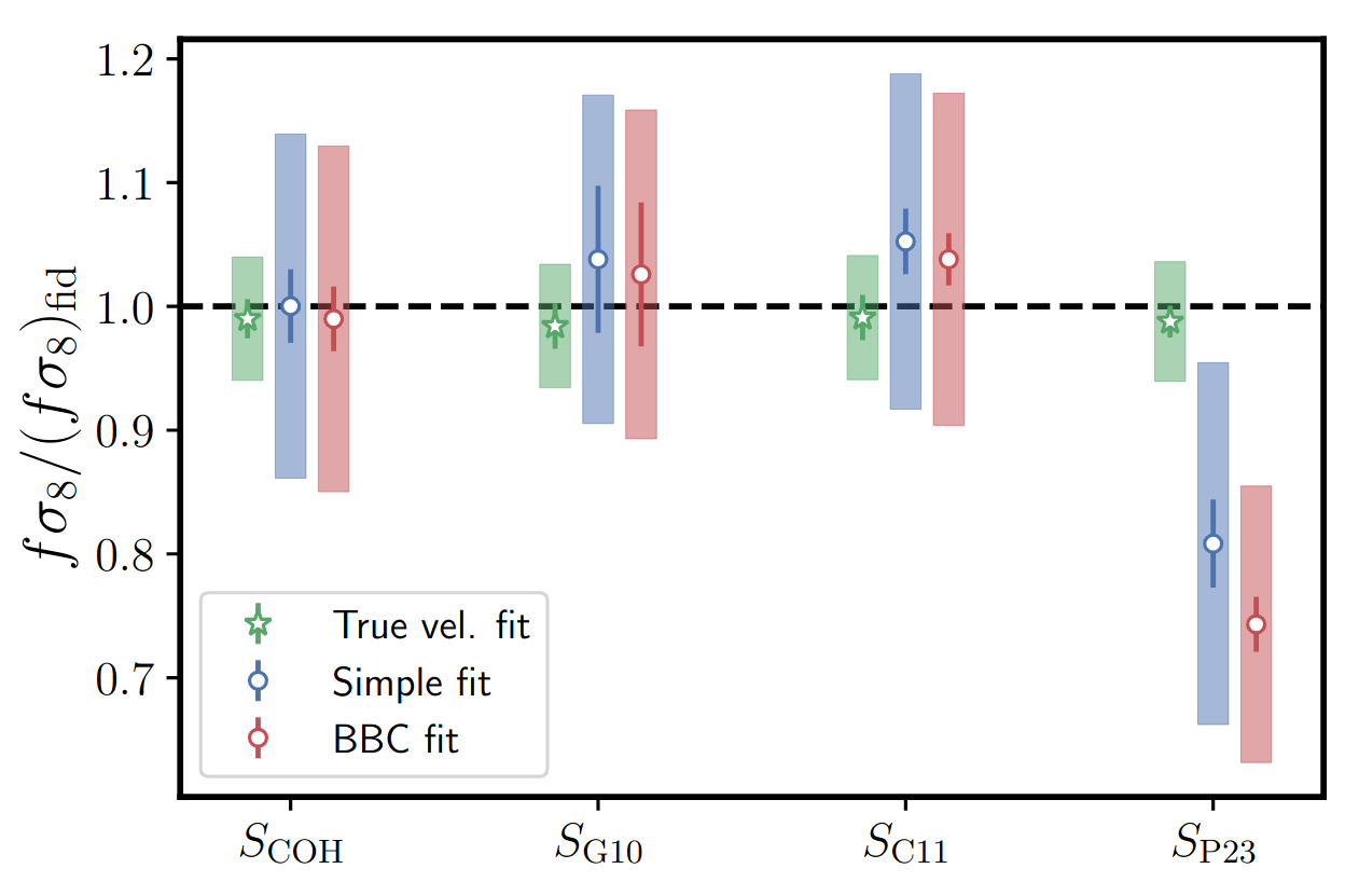
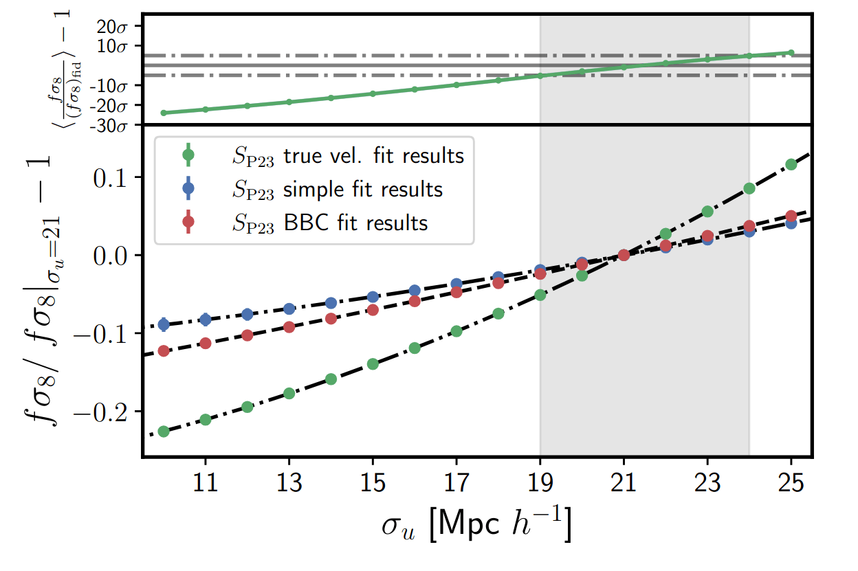
Carreres et al. 2025
Corentin Ravoux Group presentation - Dec. 2025
LSST PV Topical team
-
Creation of a new topical team under the DESC-TD WG
-
Planned projects:
-
Project 1: Modeling LSST's detection efficiency and photometric accuracy for bright targets.
-
Project 2: Analyzing filter non-uniformity over focal plane
-
Project 3: Evaluating initial forecasts against the DP1 observing logs
-
Project 4: Cross-observatory alerts
-
Project 5: Velocity-field inference bias using mocks
-
Project 6: Compile a list of methodologies used to infer f𝛔8, tabulate (dis)advantages for clear comparison
-
Project 7: Develop estimators, covariance matrix formulae, validate higher-order statistics
-
Corentin Ravoux Group presentation - Dec. 2025
Summary of PV estimations on realistic simulations
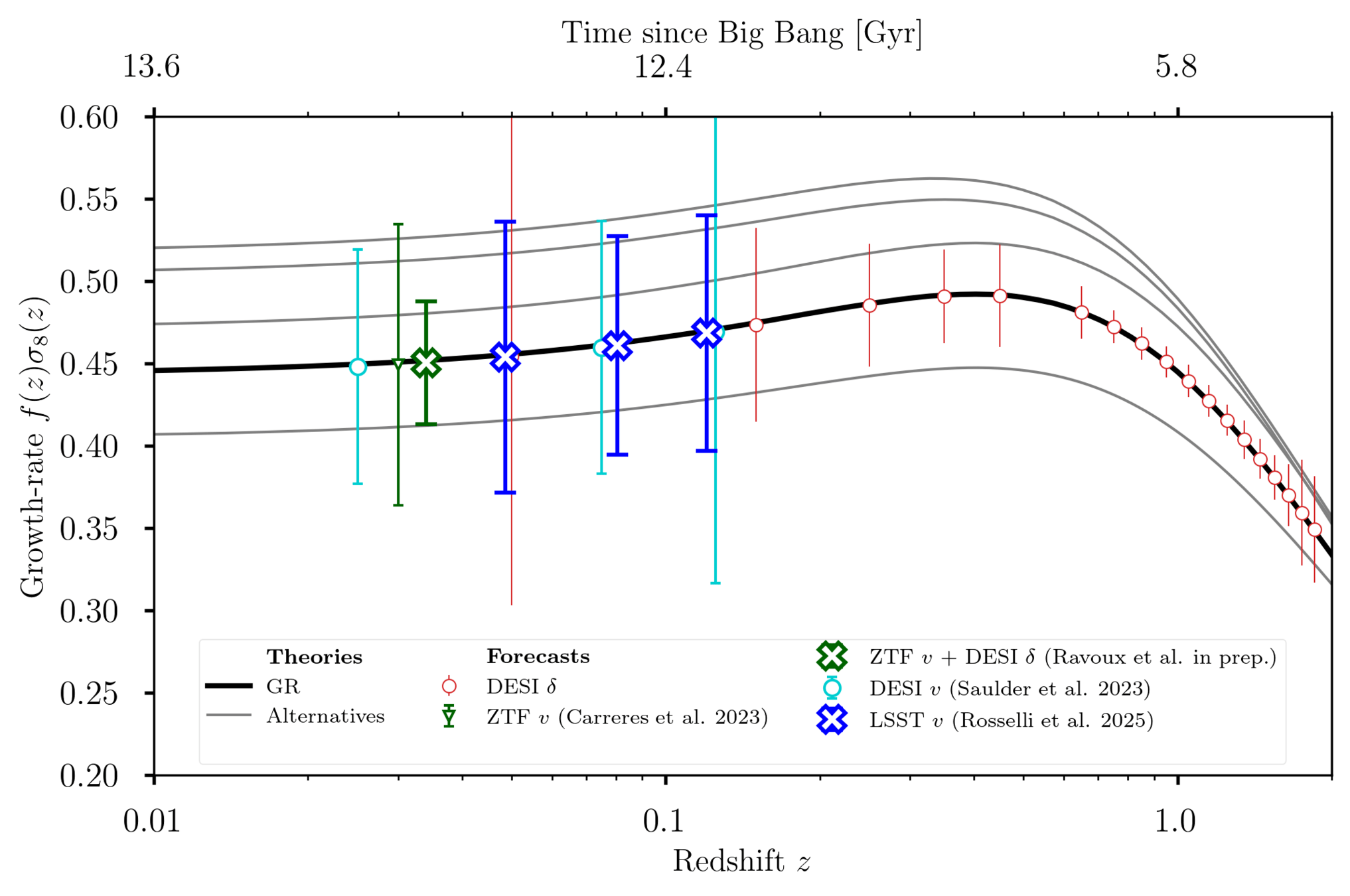
ZTF + DESI
(this talk)
ZTF (Carreres et al. 2023)
LSST (Rosselli et al. 2025)
Corentin Ravoux Group presentation - Dec. 2025
Conclusion
- Large modeling and simulation preparatory work for ZTF, LSST and combination with DESI density field
- Dedicated sofware for simulation (snsim, skysurvey) and analysis (flip)
-
Next steps:
- Application on data (Pantheon+, ZTF, DEBASS, ATLAS)
- Simulation of all-sky combination (LSST/4HS+4MOST, ZTF+DESI)
- Combination with other velocity tracers (DESI TF, FP)
ACCEL² simulation
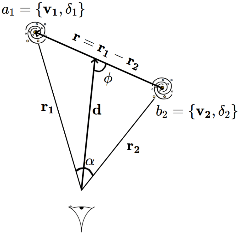
A word on wide-angle in clustering
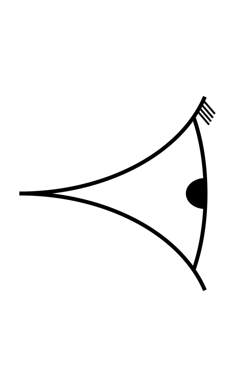

Plane parallel models
Wide angle models
Plane parallel model
- Express power spectrum model in a general way:
- vv "simple" example:
Parameters to fit
Terms to integrate analytically
Power spectra terms to integrate numerically
Plane parallel model
- Without loosing generality we can express the covariance:
Plane parallel model
Linear sum of matrix with parameters to fit as coefficients
- Without loosing generality we can express the covariance:
Plane parallel model
Hankel transform
- Most important part: Algorithmically optimized way to compute power spectrum integral, with FFTLog algorithm
- Without loosing generality we can express the covariance:
Plane parallel model
- Without loosing generality we can express the covariance:
Terms pre-computed analytically with symbolic code generaltion
- More complicated formalism derived and implemented for wide-angle
Wide angle model
linear sum of matrix
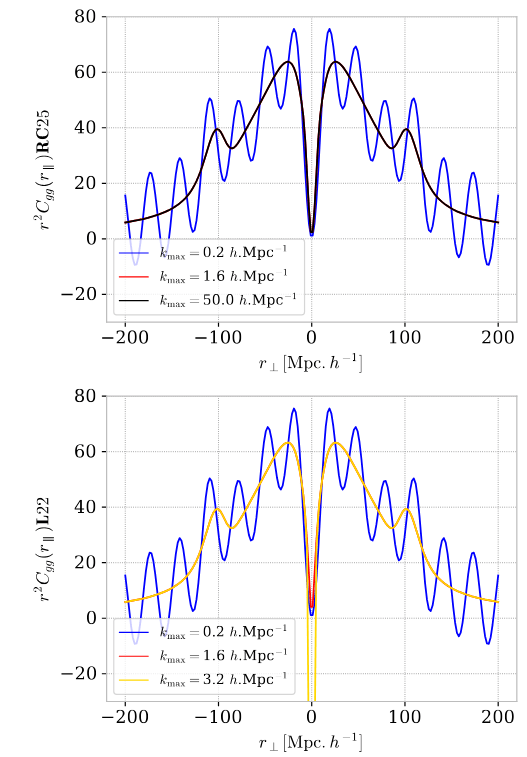
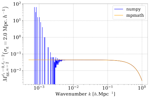
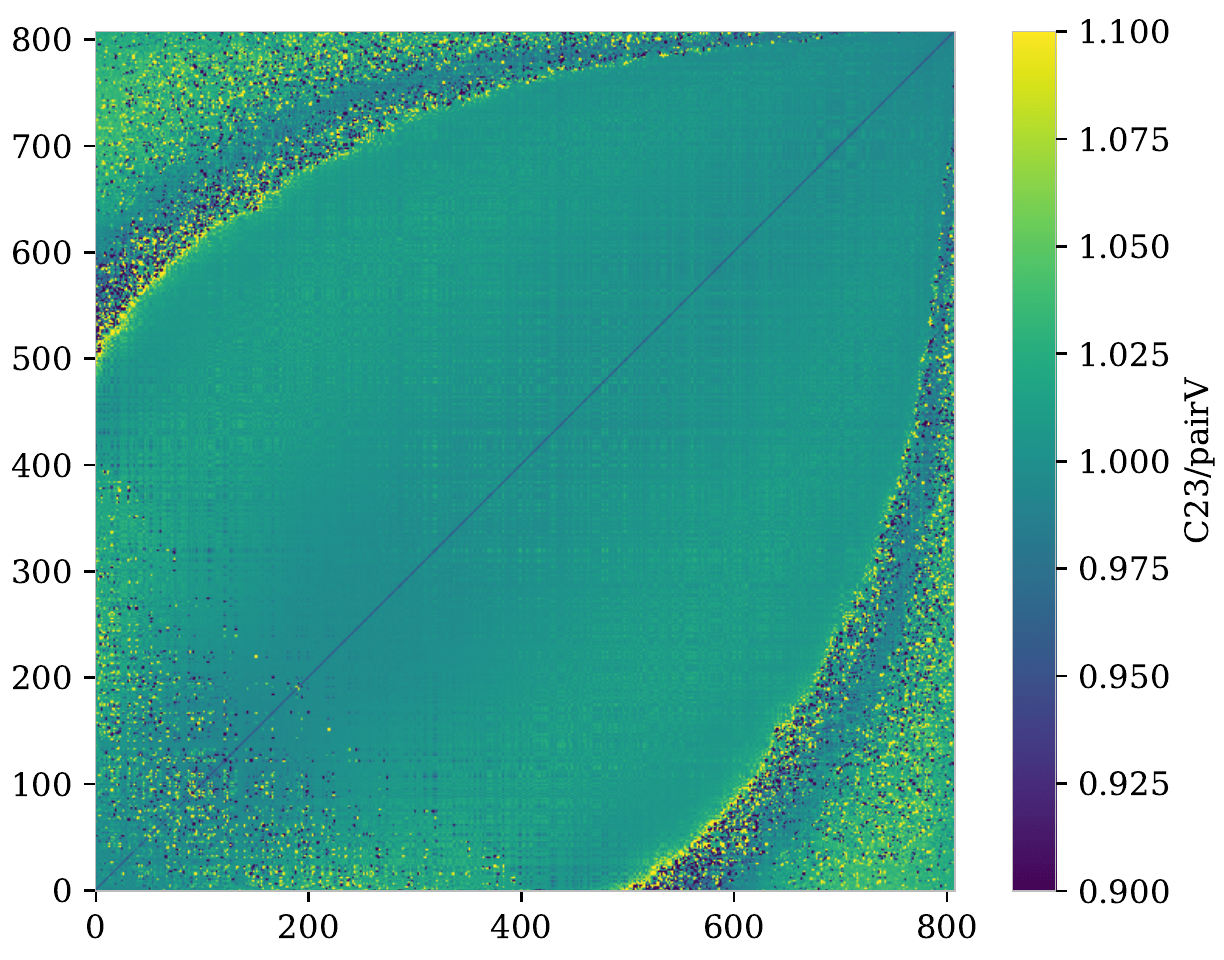
flip validations
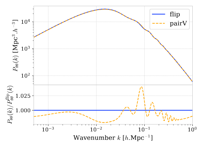
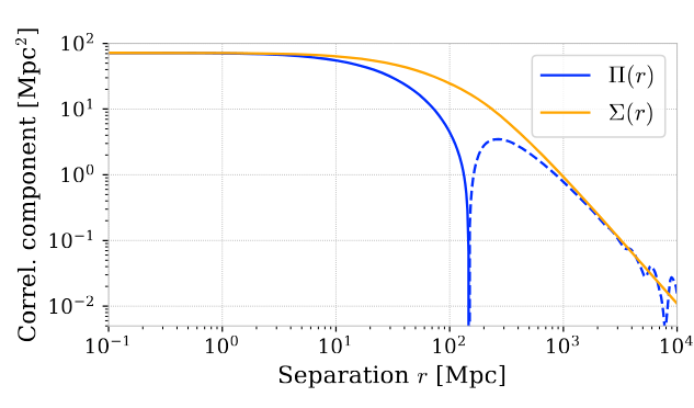
- Field covariance comparison with pairV Anthony Carr & David Parkinson
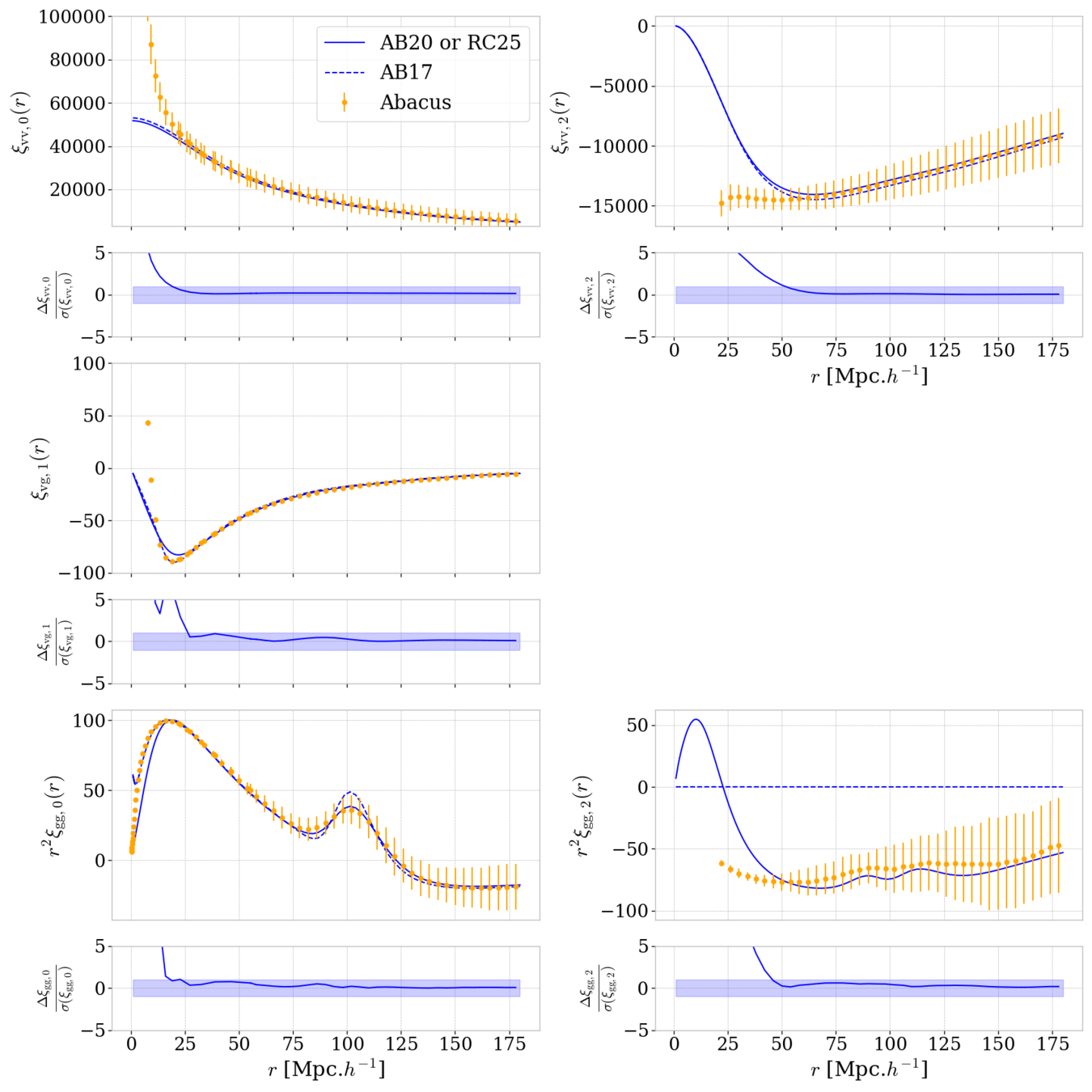
- Model validated on N-body simulations Tyann Dummerchat
Disagreement due to different power spectrum model
Ravoux et al. 2025
Ravoux et al. 2025
Survey dependent Fisher forecast
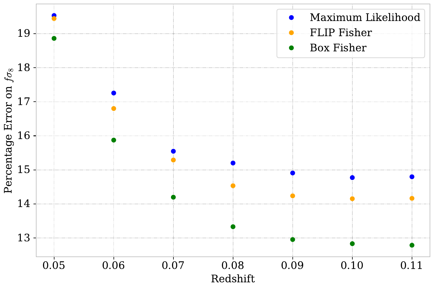
- Field covariance matrix accounts for survey geometry
- Comparing ZTF simulation (Carreres et al. 2023) with Fisher forecasts
- Error ~ 30% closer to likelihood-based than standard Fisher
Howlett et al. 2017
Ravoux et al. 2025
ZTF results
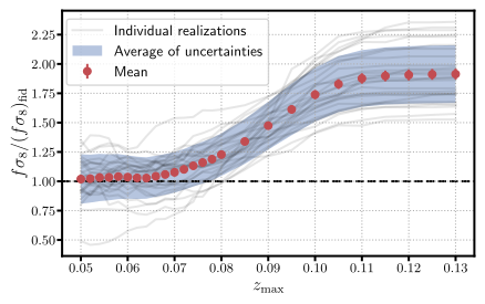
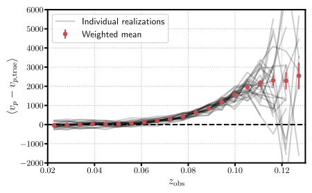
- SN Ia selection bias causes velocity & fσ8 bias at high redshift
- No fσ8 error bar improvement even with correction
- Maximum redshift usable:
Carreres et al. 2023
Carreres et al. 2023
ZTF results
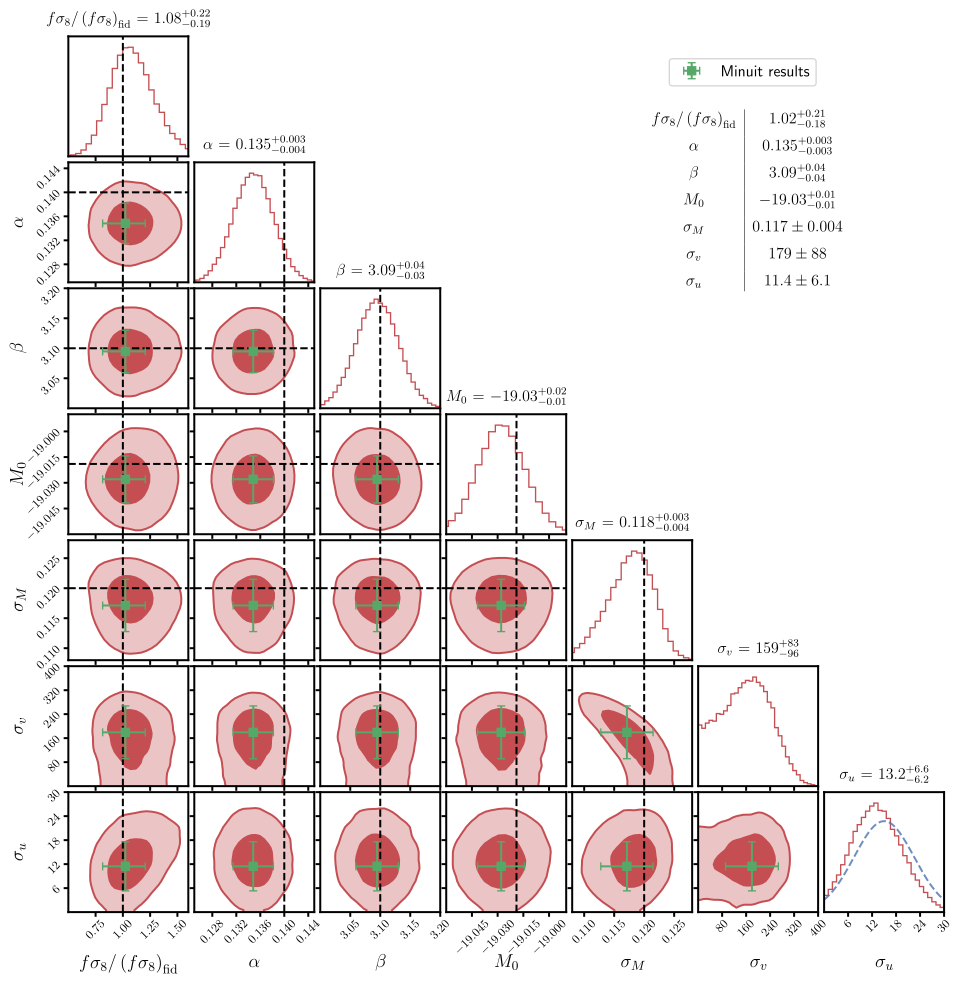
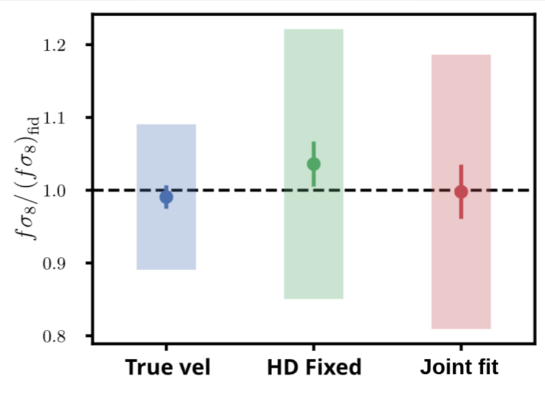
- fσ8 fit performed with Hubble diagram parameters
- no fσ8 bias on the 27 simulations
- 19 % precision measurement with only 1600 SNe Ia
Carreres et al. 2023
Carreres et al. 2023
LSST results
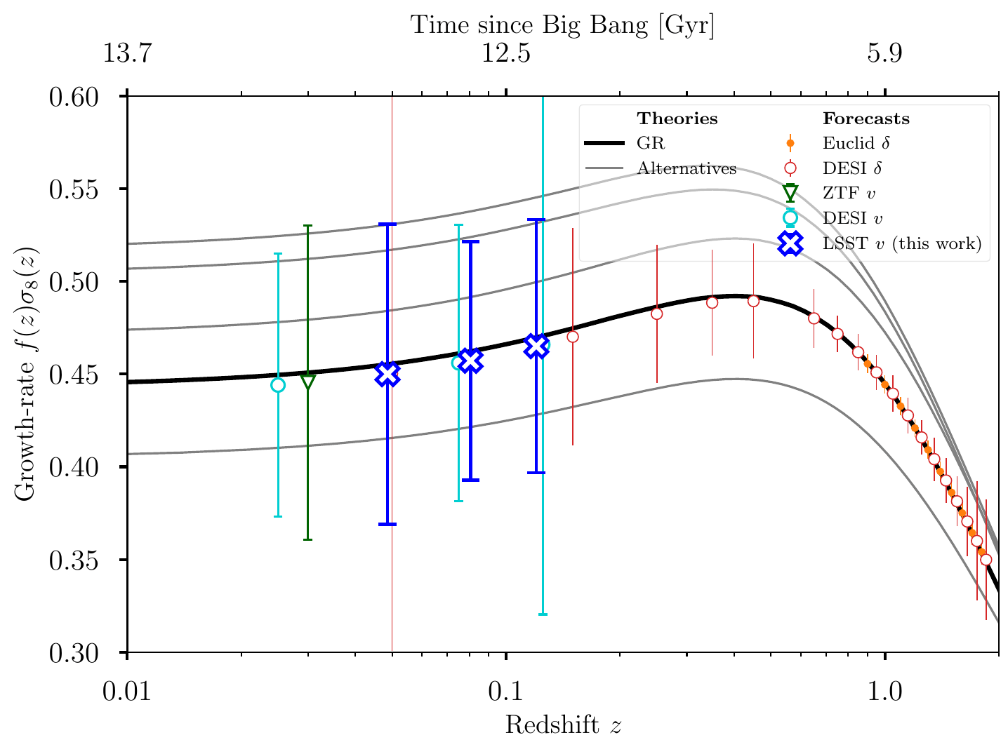
- Unbiased fσ8 measurement with full Hubble diagram fit over 3 redshift points
- How can we do better ? Combine with density field
Rosselli et al. 2025