Flip software and applications


DESC PV workshop 2025


ACCEL² simulation
Corentin Ravoux - CNRS/LPCA Clermont-Ferrand


with Bastien Carreres, Damiano Rosselli, Julian Bautista, Alex Kim and many others

Likelihood-based field-level estimator

\begin{aligned} \mathcal{L}(p) \propto & \exp\left[-\frac{1}{2} v^T(p) C_{vv}(p)^{-1} v(p)\right] \\ \end{aligned}

Velocity from SNe Ia

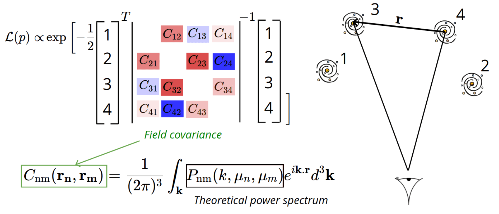
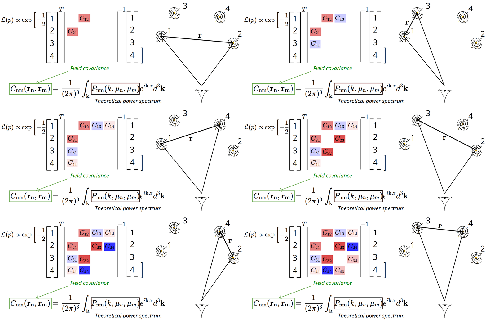
Field covariance matrix computed from theory and coordinates

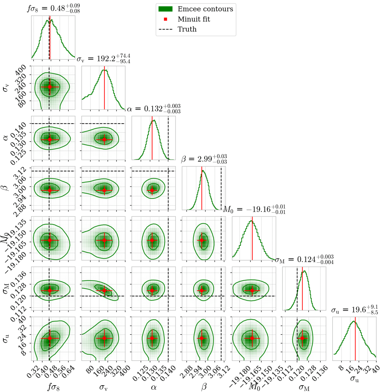
Parameters

Velocity example:

  • Purpose: Maximizing or sampling a likelihood computed from all coordinates of the data
  • p = fitted parameters: simultaneously cosmology (fσ8) and field parameters (e.g., Hubble diagram parameters α, β, M0 for SN)

Corentin Ravoux                                                                                                                                                              DESC PV workshop - September 22

Computing the field covariance
Corentin Ravoux                                                                                                                                                              DESC PV workshop - September 22

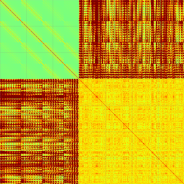
Combining densities (RSD) and peculiar velocities

\begin{aligned} \mathcal{L}(p) \propto & \exp\left[-\frac{1}{2} \right. \end{aligned}

Velocities

Density field from galaxy surveys

Full field covariance matrix
\delta
\delta
v
v
\Bigg]
-1
T
\left(C_{gg}\right)
\left(C_{gv}\right)
\left(C_{vv}\right)
\left(C_{gv}\right)

Corentin Ravoux                                                                                                                                                              DESC PV workshop - September 22

General covariance calculation

  • Objective: Improve/Extend the likelihood-based modeling
  • General form of field power spectrum
  • Algorithmically-oriented calculations (Hankel transforms)
  • Wide-angle effect accounted in the integration
C_{\mathrm{ab}}(\mathbf{r_a}, \mathbf{r_b}) = \frac{1}{(2 \pi)^3} \int_{\mathbf{k}} P_{\mathrm{ab}}(k, \mu_{\mathrm{a}}, \mu_{\mathrm{b}}) e^{i \mathbf{k}.\mathbf{r}} d^3 \mathbf{k}
P_{\mathrm{ab}}(k, \mu_{\mathrm{a}}, \mu_{\mathrm{b}}) = \sum_{n} w_{\mathrm{ab},n} F_{\mathrm{ab},n} (k, \mu_{\mathrm{a}}, \mu_{\mathrm{b}}) \mathcal{P}_{\mathrm{ab},n}(k)

gg, gv, vv

Parameters to fit

Terms to integrate analytically

Power spectra terms to integrate numerically

Corentin Ravoux                                                                                                                                                              DESC PV workshop - September 22

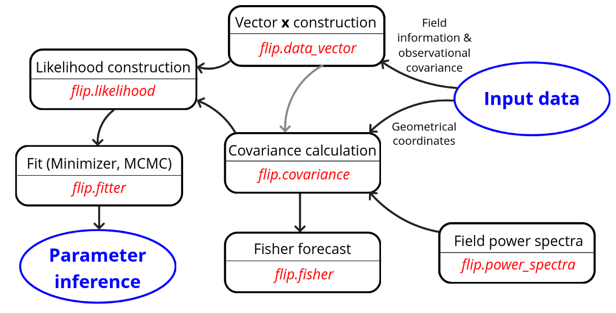
flip Field Level Inference Package

  •  python package for likelihood-based field-level inference:


https://github.com/corentinravoux/flip

  • Symbolic code generation for covariance model
  • Fast generation of field covariance
  • MCMC and Minuit fitter
  • General expression for vectors (SNIa, density, log distance...)
  • Survey geometry-dependent Fisher forecast
  • Covariance model evaluation

Flip article: arxiv:2501.16852

Contributors: Bastien Carreres, Damiano Rosselli and Alex G. Kim

Corentin Ravoux                                                                                                                                                              DESC PV workshop - September 22

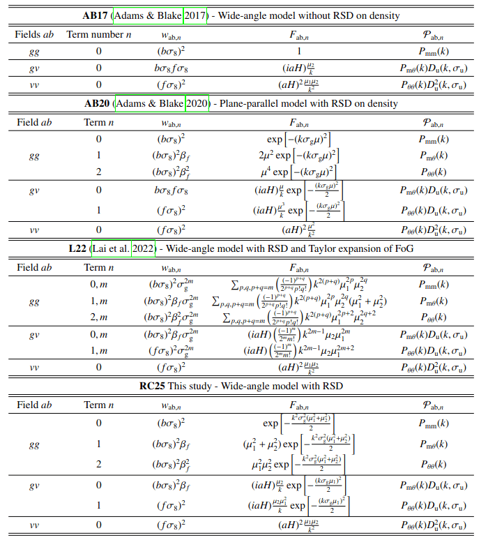
Field covariance models
Ravoux et al. 2025

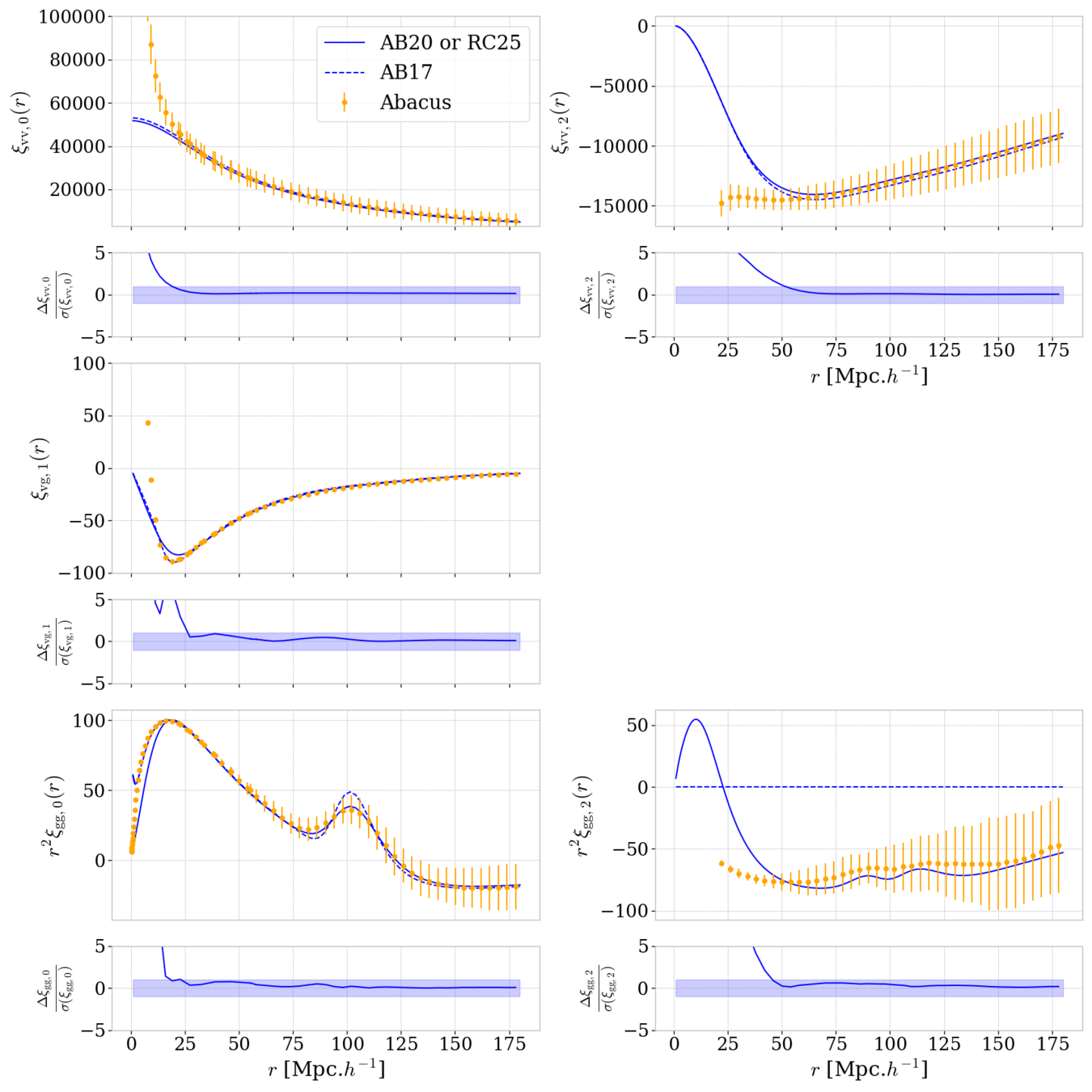
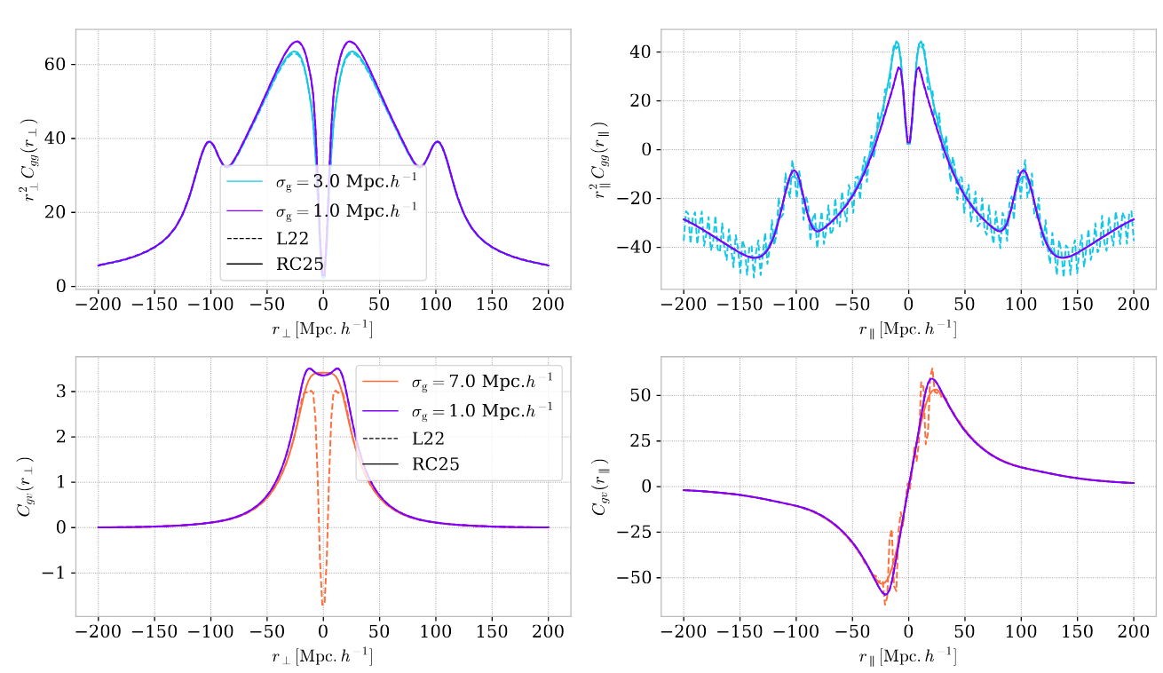
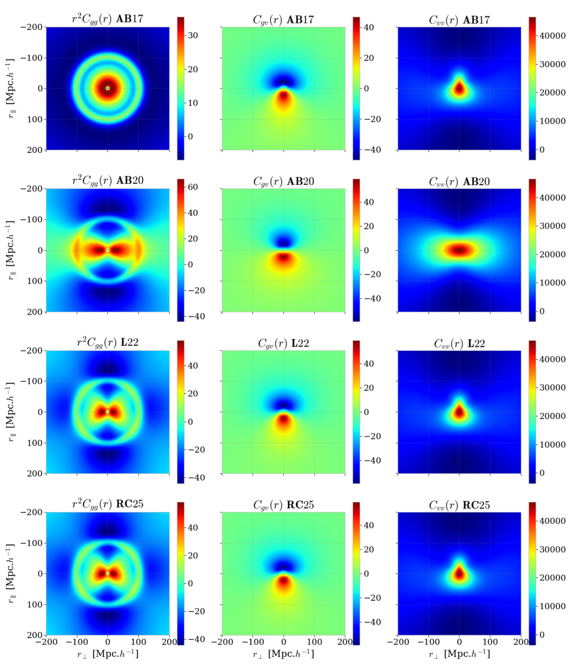
  • Model comparison on a regular coordinate grid (Adams & Blake 2017, Adams & Blake 2020, Lai et al. 2022)


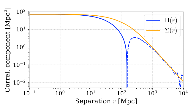
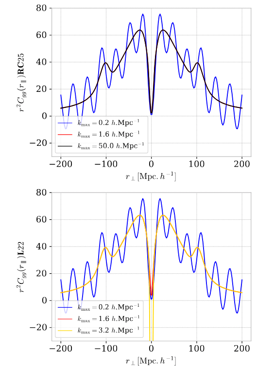
  • New wide-angle model developed (RC25): improved stability in integration and for wider fitting parameter ranges

Corentin Ravoux                                                                                                                                                              DESC PV workshop - September 22

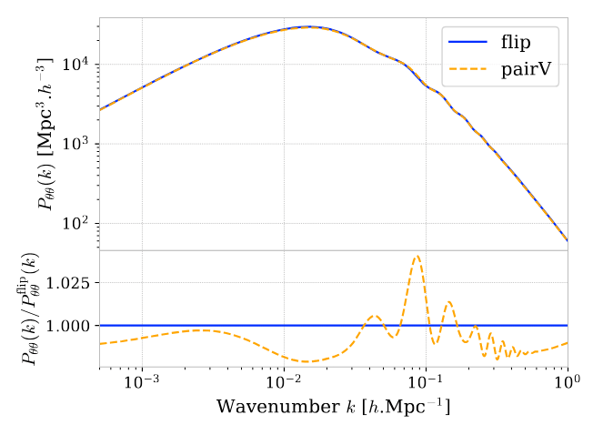
Validating flip

  • Field covariance comparison with pairV Anthony Carr & David Parkinson
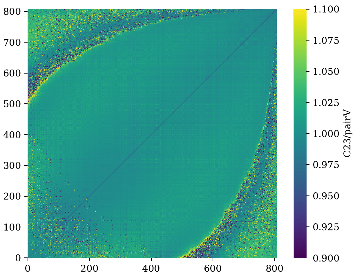
  • Model validated on N-body simulations  Tyann Dummerchat

Disagreement due to different power spectrum model

Corentin Ravoux                                                                                                                                                              DESC PV workshop - September 22

Survey dependent Fisher forecast
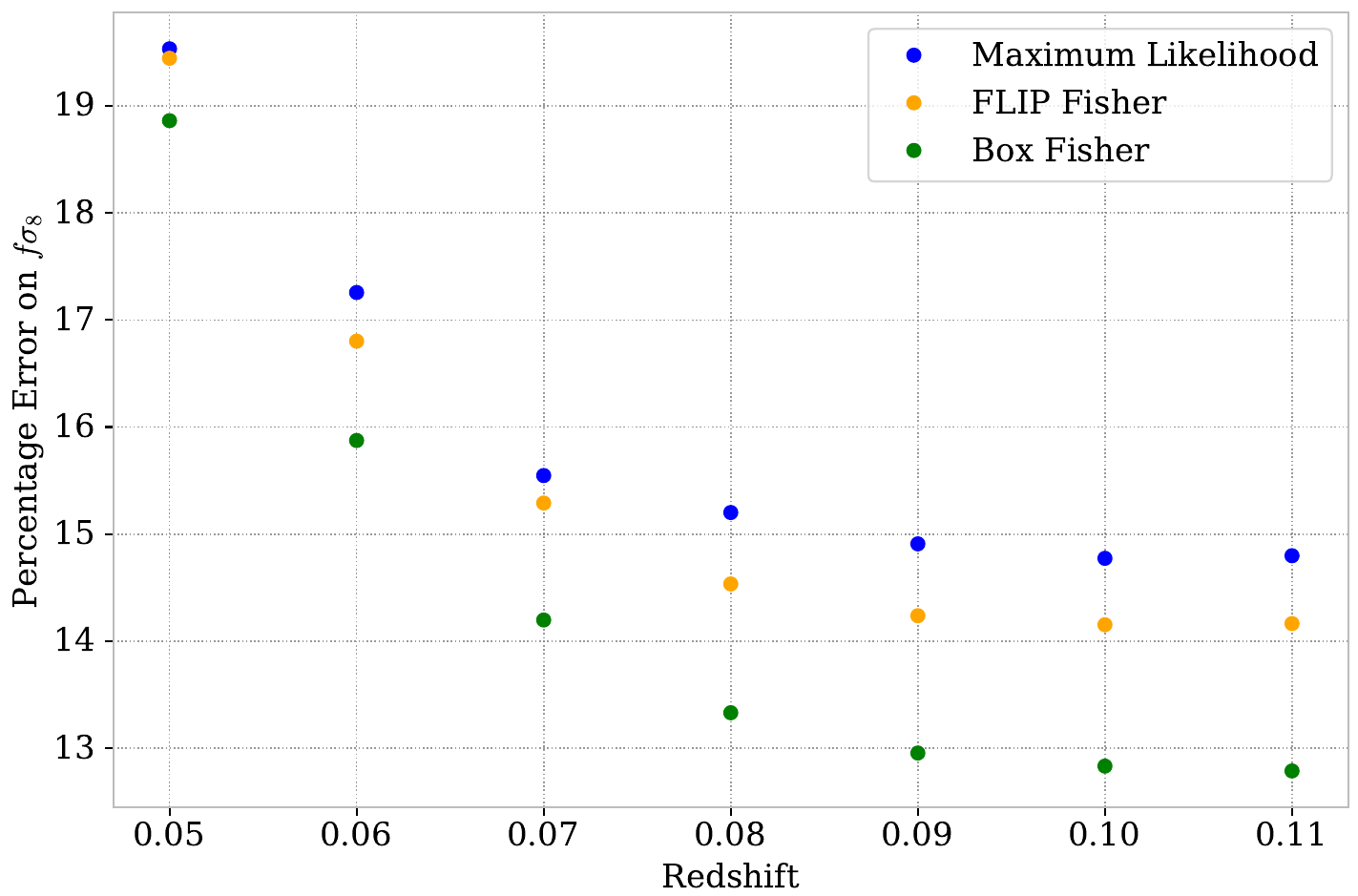
  • Field covariance matrix accounts for survey geometry
  • Comparing ZTF simulation (Carreres et al. 2023) with Fisher forecasts
  • Error ~ 30% closer to likelihood-based than standard Fisher

Damiano Rosselli

Howlett et al. 2017

Corentin Ravoux                                                                                                                                                              DESC PV workshop - September 22

Application: combining DESI galaxy density and ZTF SNIa velocities on simulation

ACCEL² simulation

Corentin Ravoux                                                                                                                                                              DESC PV workshop - September 22

Galaxy field

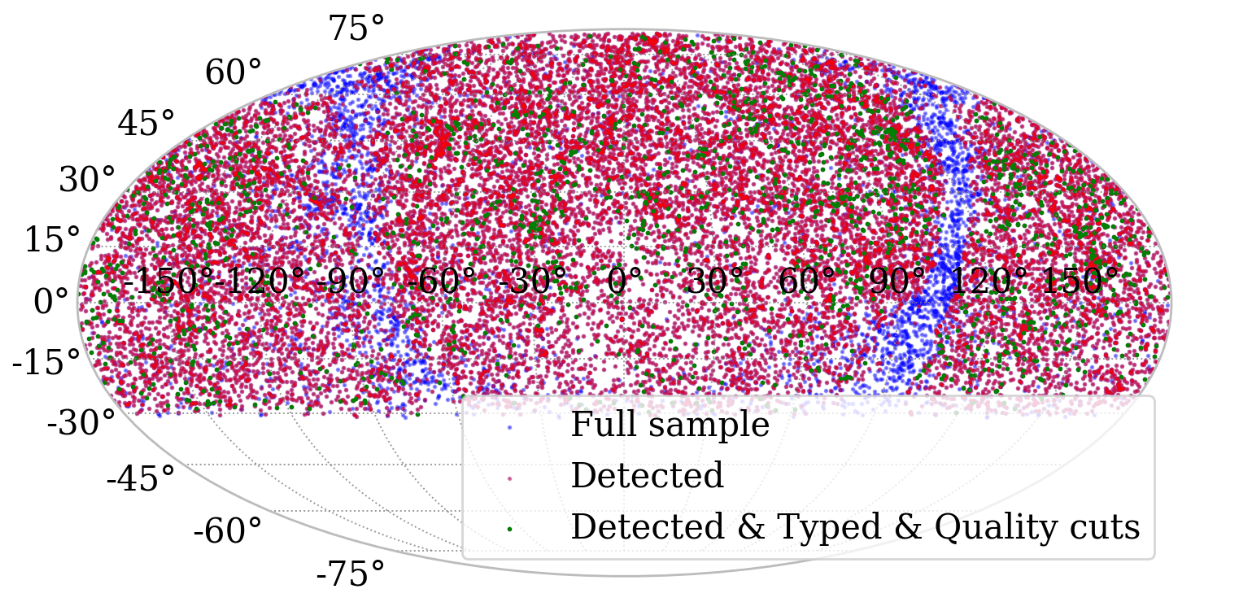
  • Runs of SNsim to mimic ZTF SNIa Y6 data set (following Carreres et al. 2023)

Supernovae velocities

https://github.com/bastiencarreres/snsim
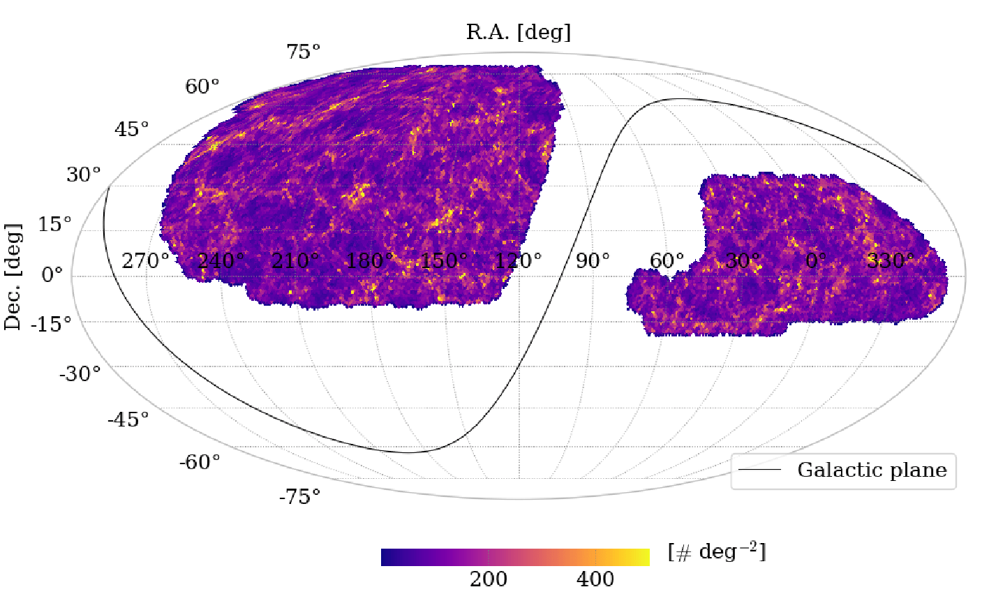
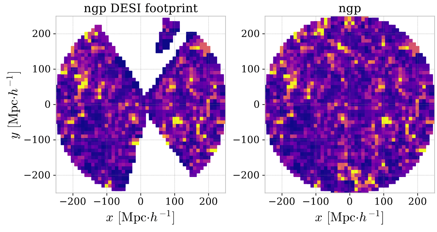
  • AbacusSummit mocks matching DESI Y5 BGS clustering and footprint
Corentin Ravoux                                                                                                                                                              DESC PV workshop - September 22

ZTF velocity fit

  • New likelihood-based model in flip
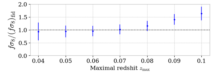
  • Velocity fit including Hubble diagram parameters (Carreres et al. 2023)


  • Variation of analysis parameters (max redshift, SNIa density...)
\hat{v}_i\left(\mathbf{p}_{\mathrm{HD}}\right)=-\frac{\ln (10) c}{5}\left(\frac{\left(1+z_i\right) c}{H\left(z_i\right) r\left(z_i\right)}-1\right)^{-1} \Delta \mu_i\left(\mathbf{p}_{\mathrm{HD}}\right)
\begin{split} \Delta \mu_i (\mathbf{p}_{\mathrm{HD}}) &=m_{B,i} - M_0 + \alpha x_{1,i} - \beta c_i \\ &- \left( 5 \log\left[(1+ z_{\mathrm{obs},i})D(z_{\mathrm{obs},i})\right] + 25 \right) \end{split}

Ravoux et al. in prep.

Corentin Ravoux                                                                                                                                                              DESC PV workshop - September 22

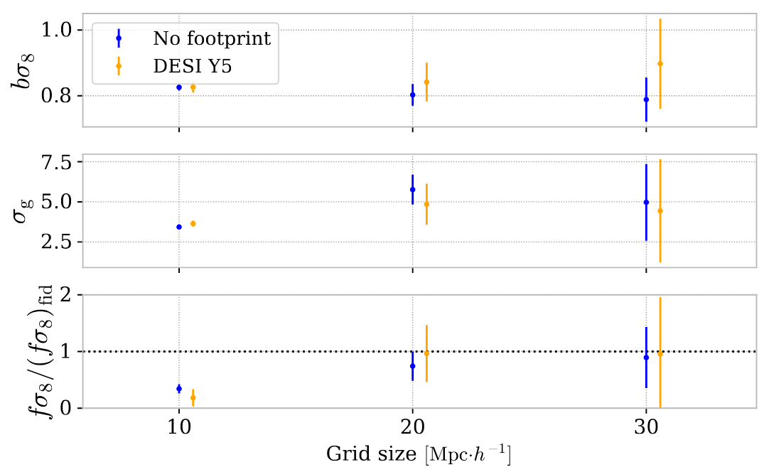
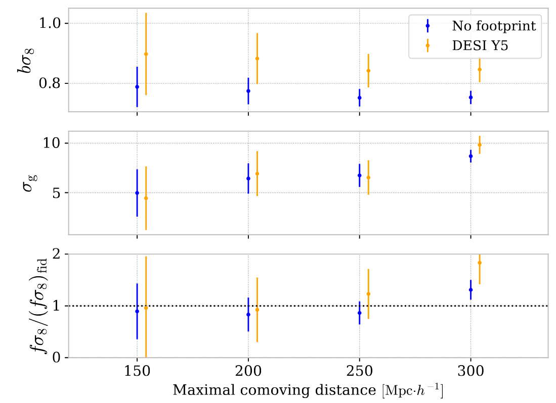
DESI density fit

  • Density grid with pypower
  • Test varying all density gridding parameters: grid size, mesh cell size, interpolation scheme (ngc, cic, tsc, pcs), footprint (Y5 or full)
  • Mean minuit fit on 27 mocks with average error bar

Ravoux et al. in prep.
Corentin Ravoux                                                                                                                                                              DESC PV workshop - September 22

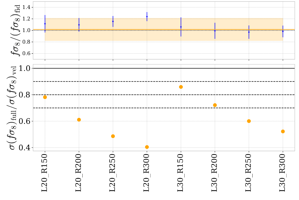
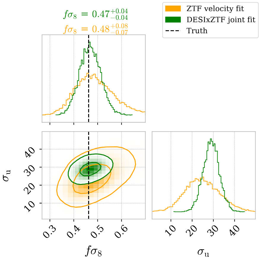
DESIxZTF joint fit

  • SNIa velocity fit with Hubble diagram parameters and density field

Adding density improves fs8 constraints up to 60%

Different density configurations

Ravoux et al. in prep.
Corentin Ravoux                                                                                                                                                              DESC PV workshop - September 22

New implementations

Corentin Ravoux                                                                                                                                                              DESC PV workshop - September 22

ACCEL² simulation

ACCEL² simulation

What is new ?

P_{\mathrm{ab}}(k, \mu_{\mathrm{a}}, \mu_{\mathrm{b}}) = \sum_{n} w_{\mathrm{ab},n} F_{\mathrm{ab},n} (k, \mu_{\mathrm{a}}, \mu_{\mathrm{b}}) \mathcal{P}_{\mathrm{ab},n}(k)

Limitating in terms of models

  • First redshift-dependent model for velocity (Alex Kim and Damiano Rosselli)
  • Introducing general redshift-dependent term (Bastien Carreres)
  • Aim: implement "no anchor"-type model
P_{\mathrm{ab}}(k, \mu_{\mathrm{a}}, \mu_{\mathrm{b}}) = \sum_{i} w_{\mathrm{ab},n} Z_{\mathrm{ab},n}(z_{\mathrm{a}}, z_{\mathrm{b}}) F_{\mathrm{ab},n} (k, \mu_{\mathrm{a}}, \mu_{\mathrm{b}}) \mathcal{P}_{\mathrm{ab},n}(k)

Corentin Ravoux                                                                                                                                                              DESC PV workshop - September 22

What is new ?

  • Needed for advanced models (EFT, gamma, no anchor...)
\mathcal{P}_{\mathrm{ab},n}(k, \Theta)

Additional parameters (cosmo or nuissance)

\Omega_{\rm m}, H_0...
\sigma_{\rm u}, \sigma_{\rm g}...

Corentin Ravoux                                                                                                                                                              DESC PV workshop - September 22

  • Emulators now implemented in flip:
    • Linear (1D, 2D)
    • Gaussian process (GPy)
    • NN implementation (torch)
    • Matrix emulators
    • Scalar emulators in development
C_{\mathrm{ab}}(\mathbf{r}_{\mathrm{a}}, \mathbf{r}_{\mathrm{b}}, \Theta) =\sum_n w_{\mathrm{ab}, n} C_{\mathrm{ab}, n}\left(\mathbf{r}_{\mathrm{a}}, \mathbf{r}_{\mathrm{b}}, \Theta \right)
P_{\mathrm{ab}}(k, \mu_{\mathrm{a}}, \mu_{\mathrm{b}}) = \sum_{n} w_{\mathrm{ab},n} F_{\mathrm{ab},n} (k, \mu_{\mathrm{a}}, \mu_{\mathrm{b}}) \mathcal{P}_{\mathrm{ab},n}(k)

Limitating in terms of models

C_{\mathrm{ab}, n}\left(\mathbf{r}_{\mathrm{a}}, \mathbf{r}_{\mathrm{b}}, \Theta \right)
\Theta

Matrix emulators

C_{\mathrm{ab}, n}\left(\mathbf{r}_{\mathrm{a}}, \mathbf{r}_{\mathrm{b}}, \Theta \right)
\mathbf{r}_{\mathrm{a}}, \mathbf{r}_{\mathrm{b}}, \Theta

Scalar emulators

Conclusion

  • flip = Framework for likelihood-based field-level inference
  • Growth rate analysis on simulation with ZTF SNIa and DESI density field
  • Next steps: improvement to non-linear models & combination with other DESI tracers (PV, TF)

ACCEL² simulation
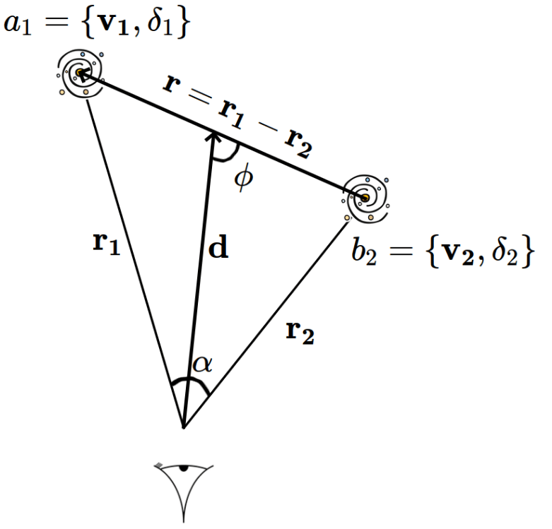
A word on wide-angle in clustering
\mathbf{r_{1}}
\mathbf{r_{2}}
\mathbf{v_{1}}
\mathbf{v_{2}}
\mathbf{r} = \mathbf{r_{1}} - \mathbf{r_{2}}

Plane parallel models

Wide angle models
\mu = \mu_1 = \mu_2
\mathbf{r_{1}}
\mathbf{r_{2}}
\mathbf{v_{1}}
\mathbf{v_{2}}
\mathbf{r} = \mathbf{r_{1}} - \mathbf{r_{2}}
\theta
\phi
\mu_1 \neq \mu_2
\mu_{i} = \mathbf{k} \cdot \mathbf{r_{i}}
\theta

Plane parallel model

  • Express power spectrum model in a general way:
P_{\mathrm{ab}}(k, \mu) = \sum_{n} w_{\mathrm{ab},n} F_{\mathrm{ab},n} (k, \mu) \mathcal{P}_{\mathrm{ab},n}(k)
  • vv "simple" example:
P_{\mathrm{vv}} = (f\sigma_8)^2 \times \left(a^2 H^2 \frac{\mu^2}{k^2}\right) \times \left(P_{\mathrm{\theta\theta}}(k) D_u^2(k, \sigma_u)\right)

Parameters to fit

Terms to integrate analytically

Power spectra terms to integrate numerically

Plane parallel model

  • Without loosing generality we can express the covariance:
C_{\mathrm{ab}}(\mathbf{r_1}, \mathbf{r_2}) = \sum_n w_{\mathrm{ab},n} \sum_{\ell} N_{\mathrm{ab},\ell}(\phi) \mathcal{H}_\ell\left[\mathcal{P}_{\mathrm{ab},n}(k)M_{\mathrm{ab},n}^{\ell}(k)\right](r)
M_{\mathrm{ab},n}^{\ell}(k) = \frac{1}{2}\int_{-1}^{1}d\mu^\prime F_{\mathrm{ab},n}(k, \mu^\prime)L_{\ell}(\mu^\prime)
N_{\mathrm{ab},\ell}(\phi) =(2\ell +1)L_\ell(\cos\left(\pi - \phi\right))

Plane parallel model

C_{\mathrm{ab}}(\mathbf{r_1}, \mathbf{r_2}) = \sum_n w_{\mathrm{ab},n} \sum_{\ell} N_{\mathrm{ab},\ell}(\phi) \mathcal{H}_\ell\left[\mathcal{P}_{\mathrm{ab},n}(k)M_{\mathrm{ab},n}^{\ell}(k)\right](r)

Linear sum of matrix with parameters to fit as coefficients

  • Without loosing generality we can express the covariance:

Plane parallel model

C_{\mathrm{ab}}(\mathbf{r_1}, \mathbf{r_2}) = \sum_n w_{\mathrm{ab},n} \sum_{\ell} N_{\mathrm{ab},\ell}(\phi) \mathcal{H}_\ell\left[\mathcal{P}_{\mathrm{ab},n}(k)M_{\mathrm{ab},n}^{\ell}(k)\right](r)

Hankel transform

\mathcal{H}_\ell\left[f(k)\right](r) = i^\ell \int_{0}^\infty\frac{k^2 dk}{2\pi^2}j_\ell(kr)f(k)
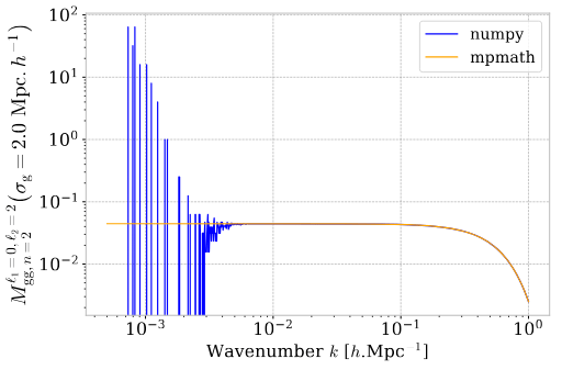
  • Most important part: Algorithmically optimized way to compute power spectrum integral, with FFTLog algorithm
  • Without loosing generality we can express the covariance:

Plane parallel model

  • Without loosing generality we can express the covariance:
C_{\mathrm{ab}}(\mathbf{r_1}, \mathbf{r_2}) = \sum_n w_{\mathrm{ab},n} \sum_{\ell} N_{\mathrm{ab},\ell}(\phi) \mathcal{H}_\ell\left[\mathcal{P}_{\mathrm{ab},n}(k)M_{\mathrm{ab},n}^{\ell}(k)\right](r)

Terms pre-computed analytically with symbolic code generaltion

  • More complicated formalism derived and implemented for wide-angle
M_{\mathrm{ab},n}^{\ell}(k) = \frac{1}{2}\int_{-1}^{1}d\mu^\prime F_{\mathrm{ab},n}(k, \mu^\prime)L_{\ell}(\mu^\prime)
N_{\mathrm{ab},\ell}(\phi) =(2\ell +1)L_\ell(\cos\left(\pi - \phi\right))