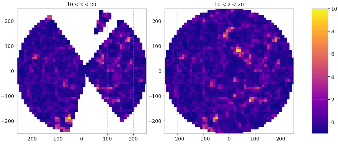
Field-level inference of growth rate

Corentin Ravoux - LPCA Clermont-Ferrand

Collaborators: Julian Bautista, Bastien Carreres, Damiano Rosseli
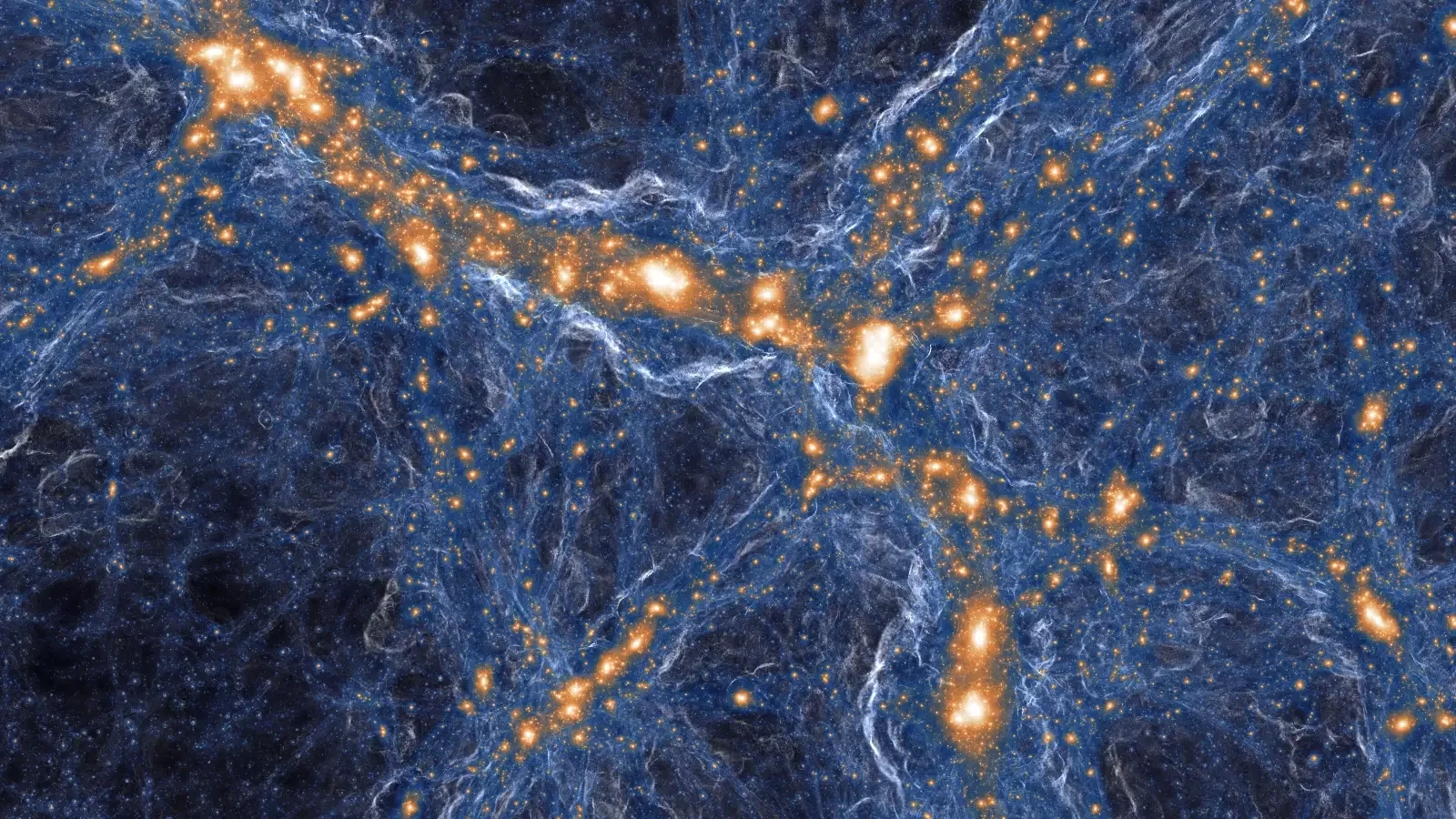
 

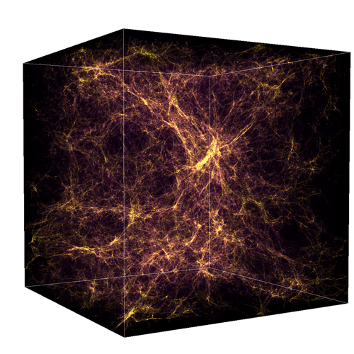
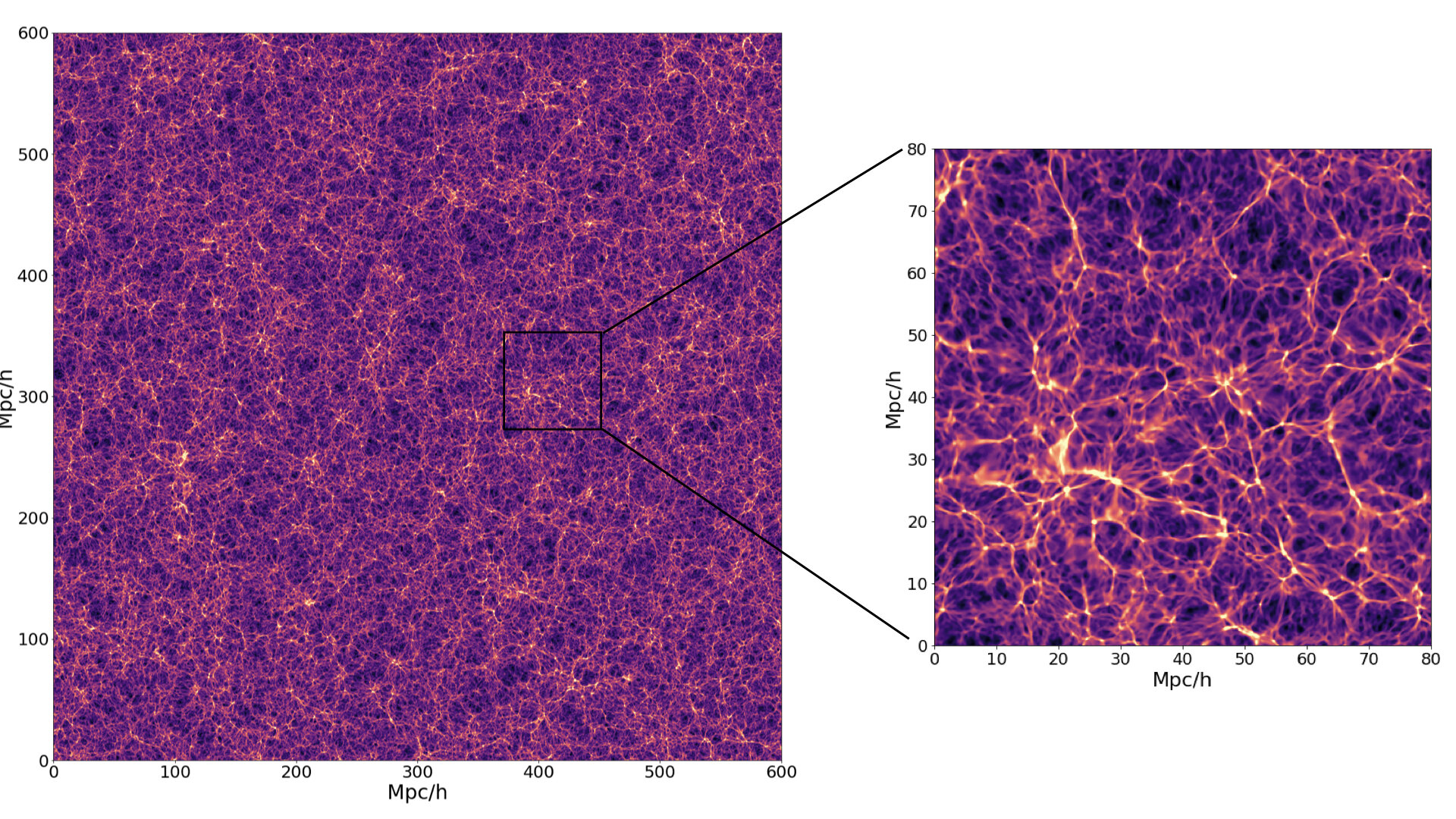
Illustris TNG simulation

Growth rate forecasts

  • RSD very effective for high-z
  • Peculiar velocities for low-z


  • Constraint improvement with combination of methods
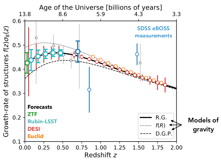
Julian's plot

Corentin Ravoux                                                                                                                                                                                 PV meeting - 26 April

Methods

  • Growth rate measurement methods with peculiar velocities:

Density/momentum power spectra

Density-velocity comparison

Forward modeling

Maximum likelihood
\langle \delta_{\mathrm{g}}(k) \delta_{\mathrm{g}}(k) \rangle
\langle \delta_{\mathrm{g}}(k) \mathbf{v}(k) \rangle
\langle \mathbf{v}(k) \mathbf{v}(k) \rangle
(\delta_{\mathrm{g}}, \mathbf{v})
\nabla \cdot \mathbf{v}_{\mathrm{pred}} \propto-a H f \delta
\mathbf{v}_{\mathrm{measured}}

Corentin Ravoux                                                                                                                                                                                 PV meeting - 26 April

Maximal likelihood estimator

\begin{aligned} \mathcal{L}(p) \propto & \exp\left[-\frac{1}{2} v^T(p) C_{vv}(p)^{-1} v(p)\right] \\ \end{aligned}

Carreres et al. 2023

peculiar velocities

Covariance matrix computed from theory and SNIa coordinates

\color{orange} f \sigma_8 \in p
  • Purpose: Minimize a likelihood computed from all coordinates of the data
  • p = parameters: contains cosmology and Hubble diagram parameters
  • Easy to include nuisance parameters

Corentin Ravoux                                                                                                                                                                                 PV meeting - 26 April

Computation of covariance matrix

P_{\mathrm{vv}} = (aHf)^2 \frac{\mu_1 \mu_2}{k^2} P_{\mathrm{\theta\theta}}(k) D_u^2(k, \sigma_u)
C_{\mathrm{vv}}(\mathbf{r_1}, \mathbf{r_2}) = \frac{1}{(2 \pi)^3} \int_{\mathbf{k}} P_{\mathrm{vv}}(k, \mu_1, \mu_2) e^{i \mathbf{k}.\mathbf{r}} d^3 \mathbf{k}

linear perturbation theory

\mu_{i} = \mathbf{k} \cdot \mathbf{r_{i}}

Estimator with wide-angle effects

\mathbf{r_{1}}
\mathbf{r_{2}}
\mathbf{v_{1}}
\mathbf{v_{2}}
\mathbf{r} = \mathbf{r_{1}} - \mathbf{r_{2}}
\theta

Corentin Ravoux                                                                                                                                                                                 PV meeting - 26 April

A word on wide-angle in clustering

\mathbf{r_{1}}
\mathbf{r_{2}}
\mathbf{v_{1}}
\mathbf{v_{2}}
\mathbf{r} = \mathbf{r_{1}} - \mathbf{r_{2}}

Plane parallel models

Wide angle models

\mu = \mu_1 = \mu_2
\mathbf{r_{1}}
\mathbf{r_{2}}
\mathbf{v_{1}}
\mathbf{v_{2}}
\mathbf{r} = \mathbf{r_{1}} - \mathbf{r_{2}}
\theta
\phi
\mu_1 \neq \mu_2
\mu_{i} = \mathbf{k} \cdot \mathbf{r_{i}}
\theta

Corentin Ravoux                                                                                                                                                                                 PV meeting - 26 April

Illustris TNG simulation

flip: coupling RSD and PV for maximum likelihood estimator

Corentin Ravoux                                                                                                                                                                                 PV meeting - 26 April

Objective

  • Improvement of growth rate measurement using simultaneously velocities and densities


  • Improvement of the python package for maximum likelihood fitting initiated by Bastien
\mathbf{r_{1}}
\mathbf{r_{2}}
\mathbf{v_{1}}
\mathbf{v_{2}}
\theta

Corentin Ravoux                                                                                                                                                                                 PV meeting - 26 April

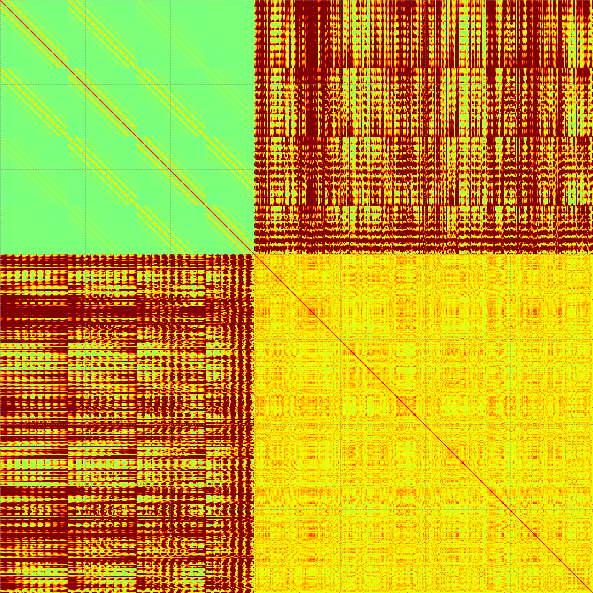
Covariance matrix

\begin{aligned} \mathcal{L}(p) \propto & \exp\left[-\frac{1}{2} \right. \end{aligned}

Velocities from SNIa (ZTF, LSST)

Density field from galaxy surveys (DESI, Euclid)

Covariance matrice computed from theory and coordinates
\delta
\delta
v
v
\Bigg]
-1
T
\left(C_{gg}\right)
\left(C_{gv}\right)
\left(C_{vv}\right)
\left(C_{gv}\right)

Corentin Ravoux                                                                                                                                                                                 PV meeting - 26 April

Linear power spectrum model with wide-angle

P_{\mathrm{vv}} = (aHf)^2 \frac{\mu_1 \mu_2}{k^2} P_{\mathrm{\theta\theta}}(k) D_u^2(k, \sigma_u)
P_{\mathrm{gg}}=\left[b^2 P_{\mathrm{mm}}(k)+b f (\mu_1^2 + \mu_2^2) P_{\mathrm{m\theta}}(k)+f^2 \mu_1^2 \mu_2^2 P_{\theta \theta}(k)\right] \exp \left[\frac{-k^2 (\mu_1^2 + \mu_2^2) \sigma_{\mathrm{g}}^2}{2}\right]
P_{\mathrm{gv}} = iaH \frac{\mu_2}{k^2} \left(bf P_{\mathrm{m\theta}}(k) + f^2 \mu_1^2 P_{\mathrm{\theta\theta}}(k) \right) \exp \left[\frac{-k^2 \mu_1^2 \sigma_{\mathrm{g}}^2}{2}\right] D_u(k, \sigma_u)
C_{\mathrm{ab}}(\mathbf{r_1}, \mathbf{r_2}) = \frac{1}{(2 \pi)^3} \int_{\mathbf{k}} P_{\mathrm{ab}}(k, \mu_1, \mu_2) e^{i \mathbf{k}.\mathbf{r}} d^3 \mathbf{k}

Very complicated (especially with the exponential term)

C_{\mathrm{gg}}, C_{\mathrm{gv}}, C_{\mathrm{vv}}

Corentin Ravoux                                                                                                                                                                                 PV meeting - 26 April

General covariance calculation

  • Objectives:
    • Test more density models
    • Possible extension to non linear corrections

Corentin Ravoux                                                                                                                                                                                 PV meeting - 26 April

vv, vg, gg

C_{\mathrm{ab}}(\mathbf{r_1}, \mathbf{r_2}) = \frac{1}{(2 \pi)^3} \int_{\mathbf{k}} P_{\mathrm{ab}}(k, \mu_1, \mu_2) e^{i \mathbf{k}.\mathbf{r}} d^3 \mathbf{k}
  • Power spectrum not expressed
  • Algorithmically-oriented calculations
  • Account for models with and without wide-angle corrections
P_{\mathrm{ab}}(k, \mu_1, \mu_2)
P_{\mathrm{ab}}(k, \mu)

Plane parallel model

C_{\mathrm{ab}}(\mathbf{r_1}, \mathbf{r_2}) = \frac{1}{(2 \pi)^3} \int_{\mathbf{k}} P_{\mathrm{ab}}(k, \mu) e^{i \mathbf{k}.\mathbf{r}} d^3 \mathbf{k}
C_{\mathrm{ab}}(\mathbf{r_1}, \mathbf{r_2}) = \sum_{\ell} i^{\ell} \int_k \frac{k^2 dk}{2 \pi^2}j_{\ell}(k r) L_{\ell}(\hat{\mathbf{d}} \cdot \hat{\mathbf{r}}) \int_{\mu = -1}^1 \frac{2 \ell+1}{2} L_{\ell}(\mu) P_{\mathrm{ab}}(k, \mu) d \mu

Using some spherical harmonic definition and multipole theorems

Corentin Ravoux                                                                                                                                                                                 PV meeting - 26 April

Plane parallel model

  • Express power spectrum model in a general way:
P_{\mathrm{ab}}(k, \mu) = \sum_{i} A_{\mathrm{ab},i} B_{\mathrm{ab},i} (k, \mu) P_{\mathrm{ab},i}(k)
  • vv simple example:
P_{\mathrm{vv}} = (f^2) \times \left(a^2 H^2 \frac{\mu^2}{k^2}\right) \times \left(P_{\mathrm{\theta\theta}}(k) D_u^2(k, \sigma_u)\right)

Parameters to fit

Terms to integrate analytically

Power spectra terms

Corentin Ravoux                                                                                                                                                                                 PV meeting - 26 April

Plane parallel model

  • Without loosing generality we can express the covariance:
C_{\mathrm{ab}}(\mathbf{r_1}, \mathbf{r_2}) = \sum_i A_{\mathrm{ab},i} \sum_l \xi_{\mathrm{ab},\ell}^{i}(r)
K_{\mathrm{ab},\ell}^i (k,\theta,\phi) = L_{\ell}(\hat{\mathbf{d}} \cdot \hat{\mathbf{r}}) \int_{\mu = -1}^1 \frac{2 \ell+1}{2} L_{\ell}(\mu) B_{\mathrm{ab},i}(k, \mu) d \mu
\xi_{\mathrm{ab},\ell}^{i}(r) = i^{\ell} \int_k \frac{k^2 dk}{2 \pi^2} P_{\mathrm{ab},i} (k) K_{\mathrm{ab},\ell}^{i} (k) j_{\ell}(k r)

Corentin Ravoux                                                                                                                                                                                 PV meeting - 26 April

Plane parallel model

C_{\mathrm{ab}}(\mathbf{r_1}, \mathbf{r_2}) = \sum_i A_{\mathrm{ab},i} \sum_l \xi_{\mathrm{ab},\ell}^{i}(r)

Parameters to fit

linear sum of matrix

  • Some insights:

Corentin Ravoux                                                                                                                                                                                 PV meeting - 26 April

Plane parallel model

  • Some insights:

Hankel transform

  • Most important part: Algorithmically optimized way to compute power spectrum integral, with FFTLog
C_{\mathrm{ab}}(\mathbf{r_1}, \mathbf{r_2}) = \sum_i A_{\mathrm{ab},i} \sum_l \xi_{\mathrm{ab},\ell}^{i}(r)

Corentin Ravoux                                                                                                                                                                                 PV meeting - 26 April

\xi_{\mathrm{ab},\ell}^{i}(r) = i^{\ell} \int_k \frac{k^2 dk}{2 \pi^2} P_{\mathrm{ab},i} (k) K_{\mathrm{ab},\ell}^{i} (k) j_{\ell}(k r)

Plane parallel model

  • Some insights:
C_{\mathrm{ab}}(\mathbf{r_1}, \mathbf{r_2}) = \sum_i A_{\mathrm{ab},i} \sum_l \xi_{\mathrm{ab},\ell}^{i}(r)

Corentin Ravoux                                                                                                                                                                                 PV meeting - 26 April

\xi_{\mathrm{ab},\ell}^{i}(r) = i^{\ell} \int_k \frac{k^2 dk}{2 \pi^2} P_{\mathrm{ab},i} (k) K_{\mathrm{ab},\ell}^{i} (k) j_{\ell}(k r)
K_{\mathrm{ab},\ell}^i (k,\theta,\phi) = L_{\ell}(\hat{\mathbf{d}} \cdot \hat{\mathbf{r}}) \int_{\mu = -1}^1 \frac{2 \ell+1}{2} L_{\ell}(\mu) B_{\mathrm{ab},i}(k, \mu) d \mu

Fully analytic calculation

Wide angle model

  • More complicated formalism derived and implemented for wide-angle


  • Conclusion:
    • Formalism can reproduce all recent covariance models (Adams & Blake 2017, Adams & Blake 2020, Lai et al. 2022, Carreres et al. 2023)
    • Start extension to other models
    • Fast with FFTLog (Hankel transform)

Corentin Ravoux                                                                                                                                                                                 PV meeting - 26 April

Wide angle model

\xi_{\mathrm{ab},\ell}^{i}(r) = \sum_j N_{\mathrm{ab},\ell}^{i,j} (\theta, \phi) \left[ i^{\ell} \int_k \frac{k^2 dk}{2 \pi^2} P_{\mathrm{ab},i} (k) M_{\mathrm{ab},\ell}^{i,j} (k) j_{\ell}(k r)\right]
C_{\mathrm{ab}}(\mathbf{r_1}, \mathbf{r_2}) = \sum_i A_{\mathrm{ab},i} \sum_l \xi_{\mathrm{ab},\ell}^{i}(r)
M_{\mathrm{ab},\ell}^{i,j=(\ell_1,\ell_2)} (k) = \int_{\mu_1 = -1}^1 \int_{\mu_2 = -1}^1 \frac{1}{4} L_{\ell_1}(\mu_1)L_{\ell_2}(\mu_2) B_{\mathrm{ab},i} (k, \mu_1, \mu_2) d \mu_1 d \mu_2
N_{\mathrm{ab},\ell}^{i,j=(\ell_1,\ell_2)} (\theta, \phi) = (4 \pi)^2 \sum_{m, m_1, m_2} G_{l, l_1, l_2}^{m, m_1, m_2} Y_{\ell m}(\hat{\mathbf{r}})^* Y_{\ell_1 m_1}(\hat{\mathbf{r_1}})^* Y_{\ell_2 m_2}(\hat{\mathbf{r_2}})^*
G_{m_1, m_2, m_3}^{l_1, l_2, l_3}=\sqrt{\frac{\left(2 l_1+1\right)\left(2 l_2+1\right)\left(2 l_3+1\right)}{4 \pi}} \left(\begin{array}{ccc} l_1 & l_2 & l_3 \\ 0 & 0 & 0 \end{array}\right)\left(\begin{array}{lll} l_1 & l_2 & l_3 \\ m_1 & m_2 & m_3 \end{array}\right)
P_{\mathrm{ab}}(k, \mu_1, \mu_2) = \sum_{i} A_{\mathrm{ab},i} B_{\mathrm{ab},i} (k, \mu_1, \mu_2) P_{\mathrm{ab},i}(k)

Corentin Ravoux                                                                                                                                                                                 PV meeting - 26 April

linear sum of matrix

flip Field Level Inference Package

https://github.com/corentinravoux/flip

  • Contains:
    • Fast generation of covariance
    • Integrated likelihood models
    • Power spectrum generator
    • Minuit and MCMC fitter
    • SNIa velocity estimate with nuissance parameters
    • Gridding routines
    • Correlation model computation

Corentin Ravoux                                                                                                                                                                                 PV meeting - 26 April

A word on symbolic calculation

  • Term integrated analytically with Sympy (python symbolic calculator)
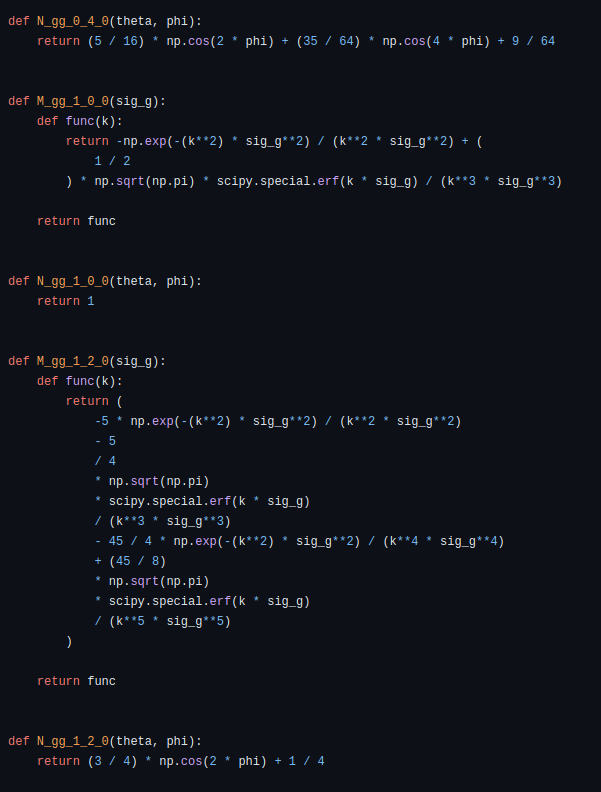
\begin{aligned} P_{\mathrm{gg}} = & \exp \left(-(k\mu \sigma_{\mathrm{g}})^2\right) \\ &[b^2 P_{\mathrm{mm}}(k) \\ & +2b f \mu^2 P_{\mathrm{m\theta}}(k) \\ &+f^2 \mu^4 P_{\theta \theta}(k)] \end{aligned}

pycode generator

Corentin Ravoux                                                                                                                                                                                 PV meeting - 26 April

K_{\mathrm{ab},\ell}^i (k,\theta,\phi) = L_{\ell}(\hat{\mathbf{d}} \cdot \hat{\mathbf{r}}) \int_{\mu = -1}^1 \frac{2 \ell+1}{2} L_{\ell}(\mu) B_{\mathrm{ab},i}(k, \mu) d \mu

Model evaluation

  • Other application: All models can be expressed as a function of separation (contraction)
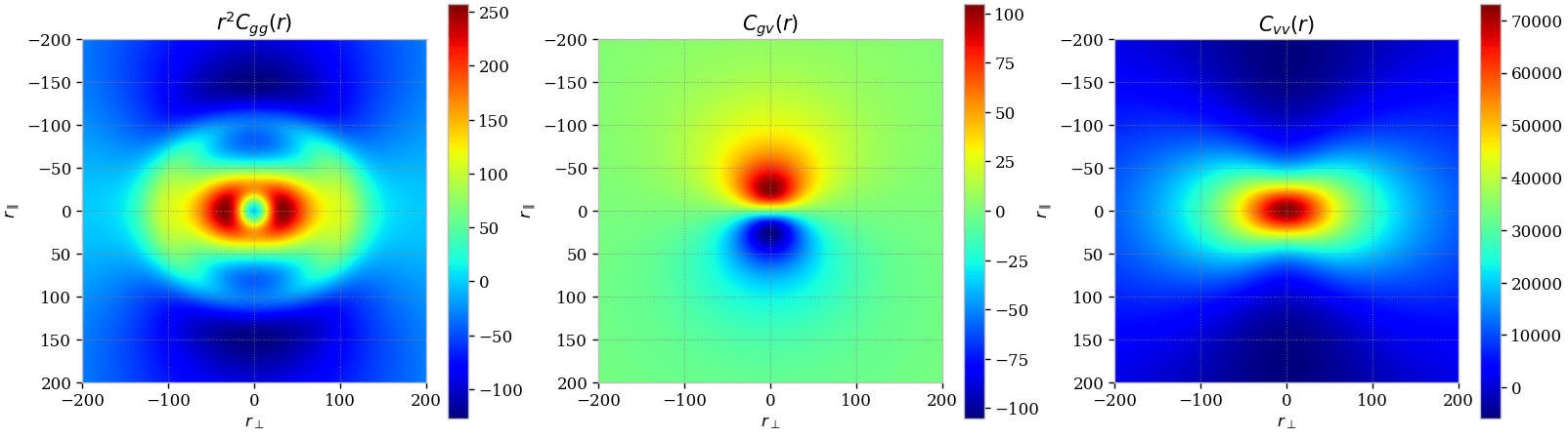
\mathbf{r} = \mathbf{r_{1}} - \mathbf{r_{2}}
r_{\parallel}
r_{\bot}

Correlation model generator with or without wide angle

Corentin Ravoux                                                                                                                                                                                 PV meeting - 26 April

What's next ?

  • Aimed improvement:
    • Unitary and end-to-end tests
    • Jax and jax_cosmo integration
    • Adding fisher forecast calculations
    • Adding likelihood models (ex: sample selection)
  • Currently: package tested on DESI/ZTF simulations and LSST simulations (Damiano, Bastien)
  • More infos:
    • Notebooks: https://github.com/corentinravoux/flip
    • Sprint: https://github.com/LSSTDESC/SprintDayWinter2024/issues/11

Corentin Ravoux                                                                                                                                                                                 PV meeting - 26 April

1

2

3

4

\mathbf{r}
\begin{aligned} \mathcal{L}(p) \propto & \exp\left[-\frac{1}{2} \right. \end{aligned}
-1

1

2

3

4

\bigg]
T

1

2

3

4

C_{12}
C_{\mathrm{nm}}(\mathbf{r_n}, \mathbf{r_m}) = \frac{1}{(2 \pi)^3} \int_{\mathbf{k}} P_{\mathrm{nm}}(k, \mu_n, \mu_m) e^{i \mathbf{k}.\mathbf{r}} d^3 \mathbf{k}
C_{13}
C_{14}
C_{21}
C_{31}
C_{41}
C_{32}
C_{42}
C_{43}
C_{24}
C_{34}
C_{23}

Theoretical power spectrum

Field covariance

Details on wide-angle

\mathbf{r_{1}}
\mathbf{r_{2}}
a_{1} = \left\{v_{1},\delta_{1}\right\}
\mathbf{r} = \mathbf{r_{1}} - \mathbf{r_{2}}
\alpha
\phi
b_{2} = \left\{v_{2},\delta_{2}\right\}
\mathbf{d}

Covariance calculation

flip.covariance

Input data

Likelihood construction

flip.likelihood

Geometrical coordinates

Vector x construction

flip.data_vector

Fit (Minimizer, MCMC)

flip.fitter

Field power spectra

flip.power_spectra

Field information & observational covariance

Fisher forecast

flip.fisher

Parameter inference